MNIST: the Hello World Example in Image Recognition
In this post we will train a simple CNN (Convolutional Neural Network) classifier in PyTorch to recognize handwritten digits in MNIST dataset.
Prerequisite
As we use PyTorch in this post, please ensure it is properly installed. In addition, we use matploblit to plot figures.
import matplotlib.pyplot as plt
import torch
import torchvision

import torch.nn as nn

print(torch.__version__)
We are referred to the PyTorch website for the installation guide[1]. For this post, it is sufficient to use the CPU version of PyTorch. For Linux, the command looks like
pip3 install torch torchvision torchaudio --index-url https://download.pytorch.org/whl/cpu
Here we declare hyperparameters for future use[4]. Their meanings will get clear in the following sections. Besides that, we manually set the random seed for reproducibility.
cfg = dict(
    n_epochs=3,
    batch_size_train=64,
    batch_size_test=1000,
    learning_rate=0.01,
    momentum=0.5,
    log_interval=10,
)
torch.manual_seed(0)
About MNIST dataset
The MNIST database (Modified National Institute of Standards and Technology database) is a large database of handwritten digits that is commonly used for training various image processing systems[2].
The torchvision package provides a convenient wrapper called
torchvision.datasets.MNIST to access MNIST dataset; see its
documentation for more details. For example, the following python
snippet can download the MNIST dataset and load it directly.
train_data = torchvision.datasets.MNIST(
    root="./data/",
    train=True,
    transform=torchvision.transforms.ToTensor(),
    download=True,
)

test_data = torchvision.datasets.MNIST(
    root="./data/",
    train=False,
    transform=torchvision.transforms.ToTensor(),
    download=True,
)
This will download MNIST dataset in the ./data/ folder if it does not
exist. In addition, the training set and test set will be loaded as
PyTorch tensors.
print(train_data)
print(f"The training dataset has shape: {train_data.data.size()}")
print(test_data)
print(f"The test dataset has shape: {test_data.data.size()}")
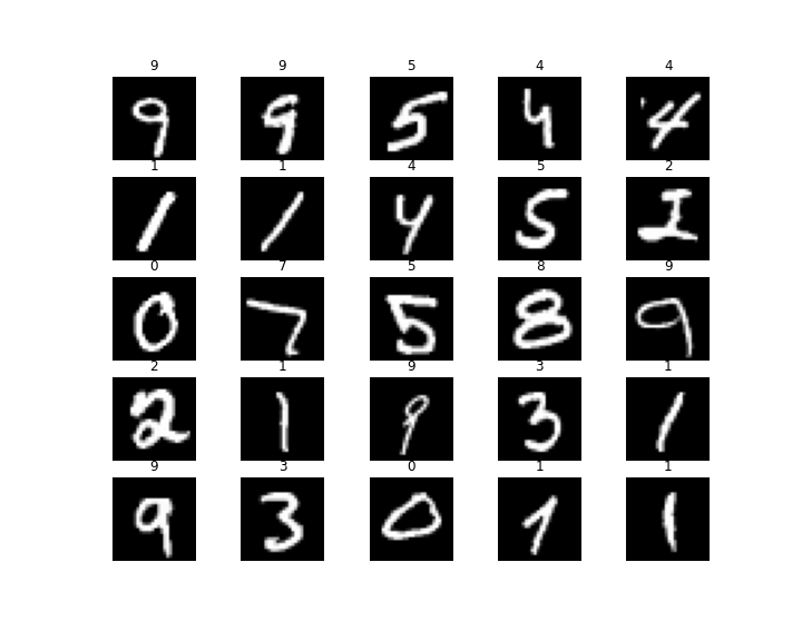
From the output, we can see that there are 60,000 training images and 10,000 test images. Each image has \(28 \times 28 = 784\) pixels. We can also look some images in the training dataset[5].
fig = plt.figure(figsize=(10, 8))
cols, rows = 5, 5
for i in range(1, cols * rows + 1):
    sample_idx = torch.randint(len(train_data), size=(1,)).item()
    img, label = train_data[sample_idx]
    fig.add_subplot(rows, cols, i)
    plt.title(label)
    plt.axis("off")
    plt.imshow(img.squeeze(), cmap="gray")
fig.savefig("./sample-images.png")
Build a CNN clasifier in PyTorch
Let \(f(x; \theta)\) be a classifier with parameters \(\theta\) which takes the data point \(x\) and predicts its label based on its function value.
By training the classifier on a dataset \(\mathcal{D}\) we roughly mean solving the optimization problem \[ \min_{\theta} \operatorname{\mathbb{E}}_{(x_i,y_i)\in \mathcal{D}} [\ell(f(x_i; \theta), y_i)]. \] Here \(y_i\) is called the label of the data point \(x_i\). In other words, minimizing the loss function \(\ell(f(x;\theta), y)\) accross all samples.
Solving this problem involves building the following parts:
- the data model \(\mathcal{D}\);
- the classifier \(f\);
- the loss function \(\ell\);
- the optimizer to find \(\min_\theta\).
data model
The crucial difference between learning and pure optimization is that the dataset of interest \(\mathcal{D}\) is unknown in a learning problem. Indeed, we cannot know the data encountered in applications and their labels before deploying our model. In most cases, we only have access to a training dataset \(\mathcal{D}_{\text{train}}\) and do our work with it. As \(\mathcal{D}_{\text{train}}\) may not fit the true data density, it is often necessary to preserve a part of it to avoid overfitting, which is called the validation dataset. Nevertheless, for the sake of simplicity we do not use this technique in this post. As the MNIST dataset provides the labels of both the training set and test set, we use the test accuracy to evaluate our model performance directly. However, it should be keep in mind that if there is no label data in the test dataset then one has to split the training dataset to construct a validation dataset manually.
We usually do a simple preprocess when loading the data, e.g., a normalization to scale the data to have mean 0 and std 1. The original mean and std of MNIST training set can be calculated easily by the following python statement.
x = torch.cat([train_data[i][0] for i in range(len(train_data))], dim=0)
print(x.mean().item(), x.std().item())
0.13066047430038452 0.30810782313346863
As we will use the idea of SGD to optimize the objective function, it is convenient to create a data loader to iteratively select a batch of data points.
train_loader = torch.utils.data.DataLoader(
    torchvision.datasets.MNIST(
        "./data/",
        train=True,
        download=True,
        transform=torchvision.transforms.Compose(
            [
                torchvision.transforms.ToTensor(),
                torchvision.transforms.Normalize((0.1307,), (0.3081,)),
            ]
        ),
    ),
    batch_size=cfg["batch_size_train"],
    shuffle=True,
)

test_loader = torch.utils.data.DataLoader(
    torchvision.datasets.MNIST(
        "./data/",
        train=False,
        download=True,
        transform=torchvision.transforms.Compose(
            [
                torchvision.transforms.ToTensor(),
                torchvision.transforms.Normalize((0.1307,), (0.3081,)),
            ]
        ),
    ),
    batch_size=cfg["batch_size_test"],
    shuffle=True,
)
Doing so allows us to use for loop to iterate the training dataset conveniently by writing
for batch_x, batch_y in train_loader:
    # do SGD with this batch of data
    pass
What happens behind this is:
- the order of samples in the dataset is shuffled before the iteration;
- each sample get preprocessed by normalizing with mean 0.1307 and std 0.3081;
- in each step, a fixed number of samples are drown from the dataset
and are stacked into
batch_xandbatch_y.
An epoch means a whole for loop and a batch means a step in the for loop.
classifier model
From the computational view, a neural network \(f(x;\theta)\) is a nested function \[ f(\cdot; \theta) = f_{N-1} \circ f_{N-2} \circ \cdots f_0,\] where each layer \(f_t\) is a parameterized function with parameter \(\theta_t\). Then the parameter \(\theta\) of the neural network \(f(x;\theta)\) is actually the collection \(\{\theta_t,\ t=0,1,\ldots, N-1\}\).
In PyTorch, a convolutional layer is a function which accepts a 4D
tensor \(x[\alpha,i,j,k]\) and outputs another 4D tensor \(y[\alpha, i',
j', k']\). The parameter of th layer consists of a bias tensor \(b[i',
j', k']\) and a weight tensor \(w[i', i, j'', k'']\). In particular, \[
y[\alpha, i'] = b[i'] + \sum_{i} w[i', i] \star x[\alpha, i],\] where
\(\star\) is the correlation operator between matrices; see also the
documention of torch.nn.Conv2d for more details. This post also
gives a review on how torch.nn.Conv2d works.
Compared to convolutional layers, fully connected layers, i.e., linear
layers in PyTorch is rather simple. They are just affine
transformations. In the most simple case, a linear layer in PyTorch
accpets a 2D tensor \(x[\alpha, i]\) and outputs another 2D tensor
\(y[\alpha, i']\). The parameter of the layer consists of a bias tensor
\(b[i']\) and a weight tensor \(w[i', i]\). In particular, \[ y[\alpha] =
b + w \circ x[\alpha], \] where \(\circ\) is the matrix-vector product.
In the general case, the index \(\alpha\) might be multiple indices and
the input \(x\) and \(y\) become high order tensors; see also the
documentation of torch.nn.Linear.
We use CNN as the basic model of our classifier[3]. In particular, the model consists of two 2D convolutional layers followed by two fully-connected layers. After each convolutional layer, there is a maximum pooling operation. In addition, the activation function is called between any two layers. We choose ReLU as our activation function.
class Net(nn.Module):
    def __init__(self):
        super().__init__()
        self.conv1 = nn.Conv2d(1, 10, kernel_size=5)
        self.conv2 = nn.Conv2d(10, 20, kernel_size=5)
        self.fc1 = nn.Linear(320, 50)
        self.fc2 = nn.Linear(50, 10)
        self.maxpool = nn.MaxPool2d(kernel_size=2)
        self.relu = nn.ReLU()

    def forward(self, x):
        x = self.relu(self.maxpool(self.conv1(x)))
        x = self.relu(self.maxpool(self.conv2(x)))
        x = x.view(-1, 320)
        x = self.relu(self.fc1(x))
        x = self.fc2(x)
        return x


clf = Net()
loss function
As we can see, the output of our model \(f(x; \theta)\) is a vector with 10 components. But how to predict the label of \(x\) and evaluate its performance? The de facto standard way is interpreting the components as the logit of the class. For example, in MNIST there are 10 classes, i.e., 10 labels in total. If the model returns \((t_0, t_1, \ldots, t_{9})\) for an image, then we say the model predicts that the probability distribution of the label \(y\) \[ \mathbb{P}(y = i) = \frac{e^{t_i}}{\sum_i e^{t_i}},\quad i=0,1,\ldots,9. \] Let \(p_i = \mathbb{P}(y=i)\) be the predicted distribution. We evaluate its performance by the relative entropy of \(p\) with respect to the true distribution \(q\), i.e., \[\ell(f(x;\theta), y) = -\sum_{i}q_i\log p_i,\] where the true distribution \(q_i\) is, of course, a deterministic distribution
$$ q_i = \begin{cases} 1,&\quad \text{$i$ is the true label},\\ 0,&\quad \text{otherwise}. \end{cases} $$
Fortunately, PyTorch provides a convenient class CrossEntropyLoss to
carry out above calculations given the predicted logits \(f(x;\theta)\)
and the true label \(y\).
loss_func = nn.CrossEntropyLoss()
optimizer
Given a pair of data \((x^{(i)}, y^{(i)})\), assume the loss of this pair is \(\phi(\tilde{y}^{(i)}, y^{(i)})\) where \(\tilde{y}^{(i)}=f(x^{(i)}; \theta)\), we want to compute the gradient of it w.r.t. \(\theta\) in order to perform gradient descent. For example, the mean-square error corresponds to \(\phi(\tilde{y}, y)=\|\tilde{y} - y\|^2\). Below is a brief summary of this post on back propagation.
Let us slightly overload the notation to denote by \(f_t(\cdot) = f(t, \cdot, \theta_t)\). Introduce the Hamiltonian \[ H(t, x, u, p) = p^\intercal f(t, x, u).\] In the calculation of the gradient, the forward phase is first executed to obtain the state variables
$$ \begin{aligned} x_0 &= x^{(i)} \\ x_{t+1} &= \nabla_p H(t, x_k, \theta_k, p)\big\vert_{p=p_{t+1}},\qquad t = 0, 1, \ldots, N-1. \end{aligned} $$Clearly, this is identical to \(x_{k+1} = f_k\circ f_{k-1}\circ \cdots f_0(x^{(i)})\). Hence, \(x_{N} = f(x^{(i)}; \theta) = \tilde{y}\) and the loss is \(\phi(x_N, y)\). The backward phase is then executed to obtain the costate variables
$$ \begin{aligned} p_N &= \partial_x \phi(x_N, y) \\ p_t &= \nabla_x H(t, x, \theta_t, p_{t+1})\big\vert_{x=x_t},\qquad t = N-1, \ldots, 1, 0. \end{aligned} $$Clearly, this is identical to \(p_{t} = (\nabla_x f_t(x_t; \theta_t))^\intercal p_{t+1}\). Here \(\nabla_x f_t\) is a Jacobian matrix and \((\nabla_x f_t)^\intercal p_{t+1}\) is often computed efficiently via Jacobian-vector product.
Finally, it is not hard to show by induction that the gradient of loss is \[ \frac{\partial}{\partial \theta_t}\phi(f(x^{(i)}; \theta), y^{(i)}) = \nabla_u H(t, x_t, u, p_{k+1})\big\vert_{u=\theta_t},\quad t=0, 1, \ldots, N-1. \]
We use the stochastic gradient descent algorithm to find the best net
parameters \(\theta\). There is no need to compute the gradient by
ourselves as PyTorch has implemented the back propagation algorithm
internally and provides various optimizers in torch.optim package. We
choose the simple SGD here.
optimizer = torch.optim.SGD(
    clf.parameters(), lr=cfg["learning_rate"], momentum=cfg["momentum"]
)
Train and test
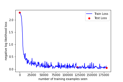
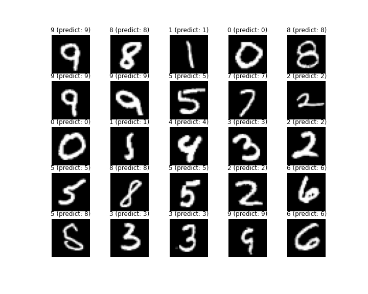
Finally, we train the model on MNIST dataset. We iterate the training set and test set several times (called epochs). In each epoch, we first train the model by going through the whole training set then test the model performance on the test set. During training process, we record the training loss after a fixed number of gradient descents. This progress is then outputed and plotted in a figure. In addition, the predicted labels of several examples are visualized.
train_losses = []
train_counter = []
test_losses = []
test_counter = [i * len(train_loader.dataset) for i in range(cfg["n_epochs"] + 1)]


def train(epoch):
    clf.train()
    for batch_idx, (batch_x, batch_y) in enumerate(train_loader):
        optimizer.zero_grad()
        logits = clf(batch_x)
        loss = loss_func(logits, batch_y)
        loss.backward()
        optimizer.step()
        if batch_idx % cfg["log_interval"] == 0:
            print(
                "Train Epoch: {} [{}/{} ({:.0f}%)]\tLoss: {:.6f}".format(
                    epoch,
                    batch_idx * len(batch_x),
                    len(train_loader.dataset),
                    100.0 * batch_idx / len(train_loader),
                    loss.item(),
                )
            )
            train_losses.append(loss.item())
            train_counter.append(
                (batch_idx * cfg["batch_size_train"])
                + ((epoch - 1) * len(train_loader.dataset))
            )


def test():
    clf.eval()
    test_loss = 0
    correct = 0
    with torch.no_grad():
        for batch_x, batch_y in test_loader:
            logits = clf(batch_x)
            test_loss += loss_func(logits, batch_y).item()
            pred = logits.data.max(1, keepdim=True)[1]
            correct += pred.eq(batch_y.data.view_as(pred)).sum()
        test_loss /= len(test_loader)
        test_losses.append(test_loss)
        print(
            "\nTest set: Avg. loss: {:.4f}, Accuracy: {}/{} ({:.0f}%)\n".format(
                test_loss,
                correct,
                len(test_loader.dataset),
                100.0 * correct / len(test_loader.dataset),
            )
        )


test()
for epoch in range(1, cfg["n_epochs"] + 1):
    train(epoch)
    test()
Test set: Avg. loss: 2.3011, Accuracy: 891/10000 (9%)

Train Epoch: 1 [0/60000 (0%)]	Loss: 2.292757
Train Epoch: 1 [640/60000 (1%)]	Loss: 2.287967
Train Epoch: 1 [1280/60000 (2%)]	Loss: 2.262003
Train Epoch: 1 [1920/60000 (3%)]	Loss: 2.230475
Train Epoch: 1 [2560/60000 (4%)]	Loss: 2.196937
Train Epoch: 1 [3200/60000 (5%)]	Loss: 2.159008
Train Epoch: 1 [3840/60000 (6%)]	Loss: 2.067780
Train Epoch: 1 [4480/60000 (7%)]	Loss: 1.874470
Train Epoch: 1 [5120/60000 (9%)]	Loss: 1.686359
Train Epoch: 1 [5760/60000 (10%)]	Loss: 1.412859
Train Epoch: 1 [6400/60000 (11%)]	Loss: 0.974901
Train Epoch: 1 [7040/60000 (12%)]	Loss: 0.792158
Train Epoch: 1 [7680/60000 (13%)]	Loss: 0.704490
Train Epoch: 1 [8320/60000 (14%)]	Loss: 0.592078
Train Epoch: 1 [8960/60000 (15%)]	Loss: 0.606974
Train Epoch: 1 [9600/60000 (16%)]	Loss: 0.503421
Train Epoch: 1 [10240/60000 (17%)]	Loss: 0.414349
Train Epoch: 1 [10880/60000 (18%)]	Loss: 0.615047
Train Epoch: 1 [11520/60000 (19%)]	Loss: 0.641742
Train Epoch: 1 [12160/60000 (20%)]	Loss: 0.359560
Train Epoch: 1 [12800/60000 (21%)]	Loss: 0.417052
Train Epoch: 1 [13440/60000 (22%)]	Loss: 0.384169
...
Train Epoch: 3 [59520/60000 (99%)]	Loss: 0.129468

Test set: Avg. loss: 0.0577, Accuracy: 9824/10000 (98%)
fig = plt.figure()
plt.plot(train_counter, train_losses, color="blue")
plt.scatter(test_counter, test_losses, color="red")
plt.legend(["Train Loss", "Test Loss"], loc="upper right")
plt.xlabel("number of training examples seen")
plt.ylabel("negative log likelihood loss")
fig.savefig("./training-curve.png")
clf.eval()

fig = plt.figure(figsize=(10, 8))
cols, rows = 5, 5
for i in range(1, cols * rows + 1):
    sample_idx = torch.randint(len(train_data), size=(1,)).item()
    img, label = train_data[sample_idx]
    with torch.no_grad():
        logits = clf(img.unsqueeze(0))
        pred = logits.data.max(1, keepdim=True)[1].item()
    fig.add_subplot(rows, cols, i)
    plt.title(f"{label} (predict: {pred})")
    plt.axis("off")
    plt.imshow(img.squeeze(), cmap="gray")

fig.savefig("./pred-sample-images.png")
Discussion
In this post, we trained a CNN classifier to recognize handwritten digits in MNIST dataset. The final test accuracy is approximately 98%. There are many ways to improve this result. For example,
- adjust hyperparameters to select a better model, including learning rate, number of training epochs, batch size, etc;
- adjust the classifier model, including adding batch normalization layer, adding dropout layer, manually initializing network parameters, etc[6, 7, 8];
- adjust the optimizer, including using other optimizing algorithm like Adam and explore their hyperparameters[9].
References
- Paszke, A., Gross, S., Massa, F., Lerer, A., Bradbury, J., Chanan, G., … Chintala, S. (2019). PyTorch: An Imperative Style, High-Performance Deep Learning Library. In Advances in Neural Information Processing Systems 32 (pp. 8024–8035)
- LeCun, Y. (1998). The MNIST database of handwritten digits. http://yann.lecun.com/exdb/mnist/
- Schmidhuber, J. (2015). Deep learning in neural networks: An overview. Neural networks, 61, 85-117.
- Koehler, G. (2020). MNIST Handwritten Digit Recognition in PyTorch. https://nextjournal.com/gkoehler/pytorch-mnist
- Nutan (2021). PyTorch Convolutional Neural Network With MNIST Dataset. https://medium.com/@nutanbhogendrasharma/pytorch-convolutional-neural-network-with-mnist-dataset-4e8a4265e118
- Ioffe, S., & Szegedy, C. (2015). Batch normalization: Accelerating deep network training by reducing internal covariate shift. In International conference on machine learning (pp. 448-456). pmlr.
- Srivastava, N., Hinton, G., Krizhevsky, A., Sutskever, I., & Salakhutdinov, R. (2014). Dropout: a simple way to prevent neural networks from overfitting. The journal of machine learning research, 15(1), 1929-1958.
- He, K., Zhang, X., Ren, S., & Sun, J. (2015). Delving deep into rectifiers: Surpassing human-level performance on imagenet classification. In Proceedings of the IEEE international conference on computer vision (pp. 1026-1034).
- Kingma, D. P., & Ba, J. (2014). Adam: A method for stochastic optimization. arXiv preprint arXiv:1412.6980.