What Happens in A Transformer Layer
Transformers serve as the backbone of large language models. Just as convolutional networks revolutionized image processing, transformers have significantly advanced natural language processing since their introduction. The efficient parallel computation and transfer learning capabilities of transformers have led to the rise of pre-trained paradigm. In this approach, a large-scale transformer-based model, referred to as the foundation model, is trained on a significant volume of data and subsequently utilized for downstream tasks through some form of fine-tuning. Our familiar friend ChatGPT is such an example, where GPT stands for generative pre-trained transformers. Meanwhile, transformer-base models achieve state-of-the-art performace for many different modalities, including text, image, video, point cloud, and audio data, and have been used for both discriminative and generative applications.
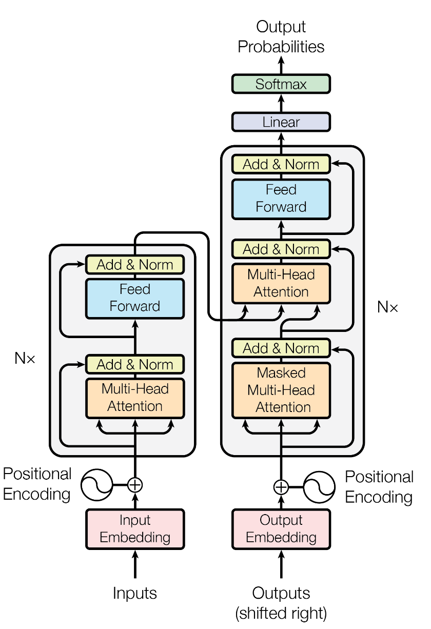
In this post, I will give a brief introduction to transformers. In particular, I will focus on the computational flow within torch.nn.TransformerEncoderLayer, outlining the process of deriving outputs from its inputs. The PyTorch implementation of transformers is based on the paper Attention is all you need by Vaswani et al. (2017). After reading this post, it should be straightforward to implement the transformer architecture from scratch. For a detailed illustration, refer to the appendix where I have included an example implementation for reference. With this knowledge, it is even possible to train a GPT given sufficient data and computational resources. For an example, check out Karpathy's nanoGPT project on GitHub.
Inputs and outputs
Similar to its predecessors, RNN and LSTM, the transformer architecture is a sequence-to-sequence model. Mathematically, it receives a sequence of vectors \(\{x_1, x_2, \ldots, x_n\}\), and returns another sequence of vectors of the same length \(\{y_1, y_2, \ldots, y_n\}\). Unlike RNN and LSTM, transformers do not compress historical information into a single hidden state vector and avoid the recurrence structure, which inherently precludes parallelization. Instead, transformers exclusively leverage the attention mechanism to explore dependencies between output and input vectors.
Notations. We use matrices to represent sequential data. For example, a sequence of vectors \(\{x_1, x_2, \ldots, x_N\}\) can be represented by a matrix \(X = (x_1, x_2, \ldots, x_N)^\intercal\), where \(x_n^\intercal\) is the \(n\)-th row vector of \(X\).
Scaled dot-product attention
The fundamental part of transformers is the attention function
\begin{equation} \operatorname{Attention}(Q, K, V) = \operatorname{Softmax}\bigl(\frac{QK^\intercal }{\sqrt{d_k}}\bigr)V, \tag{1} \end{equation}where \(\operatorname{Softmax}[X]\) is an operator that ensures each row vector of \(X\) sums up to one.
Let's explain what happends here. The inputs and output of this attention function are all matrices, where
- \(Q\) is a \(N \times d_k\) matrix, referred to as the query matrix;
- \(K\) is a \(M \times d_k\) matrix, referred to as the key matrix;
- \(V\) is a \(M \times d_v\) matrix, referred to as the value matrix;
- the output is a \(N \times d_v\) matrix.
For each row \(q_n^\intercal\) in \(Q\), we compute the similarity between it and all row vectors of \(K\),
\begin{equation} a_{nm} = \frac{q_n^\intercal k_m}{\sqrt{d_k}}, \quad m=1, 2, \ldots, M. \tag{2} \end{equation}After normalizing this set of coefficients to sum to one by the softmax function, the returned vector is a linear combination of row vectors of \(V\)
\begin{equation} y_n = \frac{1}{Z_n} \sum_m e^{a_{nm}} v_m, \quad Z_n = \sum_m e^{a_{nm}}. \tag{3} \end{equation}The final output is a matrix with the same number of rows as \(Q\), and \(y_n\) is the row vector of the output which corresponds to the input row vector \(q_n\).
Equation (1) is called scaled dot-product attention because it applies the scaled dot-product to measure the similarity between query vectors and key vectors. Imagine that for a given query \(q_n\), if there are three key vectors \(k_1, k_3\) and \(k_5\) that have the most responses, then the attention function returns a linear combination of the corresponding value vectors \(v_1, v_3\) and \(v_5\) where the coefficients are proportional to the similarities.
Self-attention and its multihead version
Self-attention is an applications of the attention function in transformers mentioned in the attention paper. It takes a sequential data \(X\) as inputs, and computes \((Q,K,V)\) in Eq. (1) by learnable linear transformations[1] of \(X\)
\begin{equation} Q = \operatorname{Linear}^Q(X), \quad K = \operatorname{Linear}^K(X), \quad V = \operatorname{Linear}^V(X). \tag{4} \end{equation}Note that these linear maps act on rows of \(X\), and thus their returns have the same number of rows (i.e., the same number of time steps) as \(X\). It is also noteworthy that these learnable linear maps are distinct from one another and each has its own set of parameters.
The self-attention can be enhanced by applying multiple attention heads. While a single attention head computes one set of \((Q, K, V)\), multihead attention computes multiple sets of these matrices using different linear maps, concatenates these outputs and applies a final linear transformation.
Take the multihead attention with 4 heads as an example. For each head \(i\), it first computes \((Q_i, K_i, V_i)\) by self-attention Eq. (4) and applies Eq. (1) to obtain the output of this head, denoted by \(H_i\). Then, it concatenates these matrices into a wider matrix \(H = [H_1, H_2, H_3, H_4]\). Finally, it applies a linear transformation to \(H\) and obtain the output.
Masks in self-attention
As a sequence-to-sequence model, it is often the case that the output vector should depend on only a subset of the vectors within the input sequence. For example, assume the input sequence is \(\{x_1, x_2, \ldots, x_N\}\) and the expected output sequence is \(\{y_1, y_2, \ldots, y_N\}\). In certain scenarios, it is imperative to ensure that generating \(y_n\) involves only the present infomation \(\{x_i\}_{i=1}^{n}\). In other words, this requirement implies that \(y_n\) should not depend on future information \(\{x_i\}_{i=n+1}^N\).
To enforce this causal constraint on self-attention, we can add a mask matrix to the similarity matrix and eliminate undesired dependence. Specifically, consider Eq. (2) and Eq. (3), which describe how to compute the output \(y_n\) from the row vectors \((q_n, k_m, v_m)\) of \((Q, K, V)\). In self-attention these vectors are obtained by linear transformations of the respective input data vectors \[ q_n = \operatorname{Linear}^Q(x_n), \quad k_m = \operatorname{Linear}^K(x_m), \quad v_m = \operatorname{Linear}^V(x_m). \] Therefore, the similarity coefficient \(a_{nm}\) in Eq. (2) relies on \(x_n\) and \(x_m\). To ensure \(y_n\) remains independent of \(\{x_i\}_{i=n+1}^N\), we need only to ensure the summation in Eq. (3) encompasses only \(1 \leq m \leq n\). By introducing a mask matrix \(b_{nm}\) and adding it to the similarity matrix, we get \[ b_{nm} := \begin{cases} 0 & \quad m \leq n \\ -\infty & \quad m > n \end{cases}, \qquad \hat{a}_{nm} := a_{nm} + b_{nm} = \begin{cases} a_{nm} & \quad m \leq n \\ -\infty &\quad m > n \end{cases}. \] Consequently, the output of the masked self-attention is \[ \hat{y}_n = \frac{1}{Z_n}\sum_m e^{\hat{a}_{nm}} v_m = \frac{1}{Z_n}\sum_{m=1}^n e^{a_{nm}} v_m, \quad Z_n = \sum_{m=1}^n e^{a_{nm}}. \] As a result, the calculation of \(\hat{y}_n\) no longer depends on future information \(\{x_i\}_{i=n+1}^N\).
The same trick can be applied to ignore the impact of <pad> tokens. In
some applications, particularly in natural language process tasks, the
input sequence is padded to a fixed length for batch
computations. Say, for example, an input sequence may look like
\(\{x_1, x_2, x_3, x_4, x_5\}\) where \(x_4\) and \(x_5\) are actually <pad>
tokens. In that case, we may want to ensure that the output \(y_n\) do
not pay attention to those <pad> tokens. We therefore introduce a mask
to restrict the summation in Eq. (3) to \(1 \leq m \leq 3\), \[ b_{nm}
:= \begin{cases} 0 & \quad m \leq 3 \\ -\infty & \quad m > 3 \end{cases},
\qquad \hat{a}_{nm} := a_{nm} + b_{nm} = \begin{cases} a_{nm} & \quad
m \leq 3 \\ -\infty &\quad m > 3 \end{cases}. \] Consequently, the output of
the masked self-attention is \[ \hat{y}_n = \frac{1}{Z_n}\sum_m
e^{\hat{a}_{nm}} v_m = \frac{1}{Z_n}\sum_{m=1}^3 e^{a_{nm}} v_m, \quad
Z_n = \sum_{m=1}^3 e^{a_{nm}}. \] As a result, the calculation of
\(\hat{y}_n\) no longer depends on <pad> tokens \(\{x_4, x_5\}\).
Transformer Layers
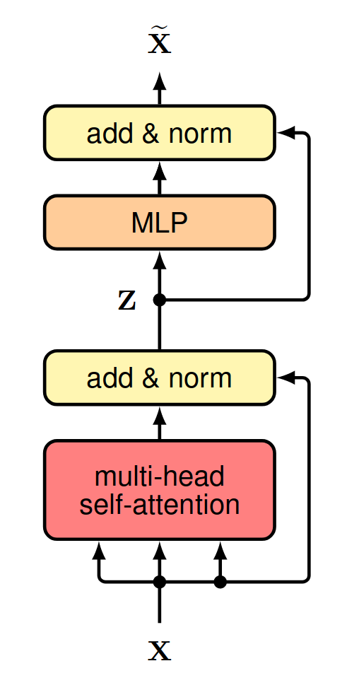
Figure 1 shows an overall architecture for a single transformer layer. It consists of two major trainable blocks, a self-attention block and a multilayer perceptron block. Each block is enclosed by a residual connection and a layer normalization; see the appendix for a brief explanation of layer normalization. The pseudocode for the forward pass is provided below.
def forward(
    self, x: torch.Tensor, mask: torch.Tensor | None = None
) -> torch.Tensor:
    """
    Forward pass of the Transformer Encoder Layer.

    Args:
    - x (torch.Tensor): Input tensor with shape (batch_size, seq_len, d_model).
    - mask (torch.Tensor, optional): Mask tensor with shape (seq_len, seq_len) or None.

    Returns:
    - torch.Tensor: Transformed output tensor with shape (batch_size, seq_len, d_model).
    """
    y = self.norm1(x)
    y = self.self_attn(y, y, y, mask=mask)
    x = x + y

    y = self.norm2(x)
    y = self.mlp(y)
    x = x + y

    return x
It is worthing noting that in this pseudocode, we employ the pre-norm configuration to wrap the blocks. This differs from the original structure in the attention paper by Vaswani et al. (2017), which takes the post-norm configuration. For a more detailed comparison between pre-norm and post-norm, please refer to the paper by Xiong et al. (2020).
The GPT-3 architecture is essentially a stack of such transformer layers, supplemented by an initial embedding layer to translate tokens into vectors and a final layer to predict tokens based on the transformer outputs.
Conclusions
The core of a transformer layer is the multi-head self-attention layer, whose inputs and outputs are both sequences. I have explained the overall computational flow step by step in the sections above, and readers should now feel comfortable with what happens in torch.nn.TransformerEncoderLayer. For demonstration purposes, a simple implementation is provided here. Lastly, it should be mentioned that the original paper used a slightly more complex architecture. For interested readers, please refer to the appendices of this post or the references listed below.
References
Books and Papers
- Bishop, C. M., & Bishop, H. (2024). Deep learning: Foundations and concepts (pp. 357-406). Springer.
- Zhang, A., Lipton, Z. C., Li, M., & Smola, A. J. (2023). Attention Mechanisms and Transformers. In Dive into Deep Learning. Cambridge University Press. https://d2l.ai/chapter_attention-mechanisms-and-transformers/index.html
- Xiong, R., Yang, Y., He, D., Zheng, K., Zheng, S., Xing, C., Zhang, H., Lan, Y., Wang, L., & Liu, T.-Y. (2020). On layer normalization in the transformer architecture. Proceedings of the 37th International Conference on Machine Learning, 119, 10524–10533. https://arxiv.org/pdf/2002.04745
- Vaswani, A., Shazeer, N., Parmar, N., Uszkoreit, J., Jones, L., Gomez, A. N., Kaiser, Ł. ukasz, & Polosukhin, I. (2017). Attention is all you need. Advances in Neural Information Processing Systems, 30. https://papers.nips.cc/paper_files/paper/2017/hash/3f5ee243547dee91fbd053c1c4a845aa-Abstract.html
Online resources (concepts)
- Kim, E., & Ashish, N. (2024). Discussion 6. In Data C182 Fall 2024. https://datac182fa24.github.io/assets/section_notes/week08_solution.pdf
- Raschka, S. (2023). About layernorm variants in the original transformer paper. https://magazine.sebastianraschka.com/p/why-the-original-transformer-figure
- Zhang, M. (2022). DIsucssion 7. In CS182/282A Spring 2022. https://datac182fa24.github.io/assets/section_notes/week09_solution.pdf
- Mongaras, G. (2022). How do self-attention masks work? Medium. https://gmongaras.medium.com/how-do-self-attention-masks-work-72ed9382510f
- Adaloglou, N. (2020). How Transformers work in deep learning and NLP: an intuitive introduction. AI Summer. https://theaisummer.com/transformer/
- Karpathy, A. (2019). A recipe for training neural networks. https://karpathy.github.io/2019/04/25/recipe/
- Alammar, J. (2018). The illustrated transformer. https://jalammar.github.io/illustrated-transformer/
Online resources (codes)
- BavalpreetSinghh (2024). Transformer from scratch using Pytorch. Medium. https://medium.com/@bavalpreetsinghh/transformer-from-scratch-using-pytorch-28a5d1b2e033
- Erdogan, E. (2024). Examining Multihead Attention. GitHub Gist. https://gist.github.com/eneserdo/77b468f61fa5c3c9f4587b4a51fca963
- Karpathy, A. (2023). Let's build GPT: from scratch, in code, spelled out [Video]. YouTube. https://www.youtube.com/watch?v=kCc8FmEb1nY&t=5722s
- PyTorch (2023). Transformer Layers. PyTorch Documentations. https://pytorch.org/docs/stable/nn.html#transformer-layers
- Karpathy, A. (2022). NanoGPT. GitHub. https://github.com/karpathy/nanoGPT
- Arunmohan003 (2022). Transformer from scratch using pytorch. Kaggle. https://www.kaggle.com/code/arunmohan003/transformer-from-scratch-using-pytorch/notebook
- CS182 HW03 (2021). Natural language processing. https://github.com/cs182sp21/hw3_public/blob/master/2%20Summarization.ipynb
- Harvard NLP (2018). The Annotated Transformer. https://nlp.seas.harvard.edu/2018/04/03/attention.html
- Lynn-Evans, S. (2018). How to code The Transformer in Pytorch. Medium. https://towardsdatascience.com/how-to-code-the-transformer-in-pytorch-24db27c8f9ec
Appendix: Layer normalization and batch normalization
Layer normalization and batch normalization are both normalization operations. The key difference is that they operate on different dimensions. Layer normalization computes the statistics accross the feature dimension, whereas batch normalization computes the statistics across the batch dimension. For example, given a batch of inputs \(x\) with a shape of \((N, C)\), where \(N\) is the batch dimension and \(C\) is the feature dimension. Layer normalization computes the mean, variance, and normalized outputs by \[ \mu_i = \frac{1}{C}\sum_j x_{ij}, \quad \sigma_i = \frac{1}{C}\sum_j(x_{ij} - \mu_i)^2, \quad \tilde{x}_{ij} = \frac{x_{ij} - \mu_i}{\sqrt{\sigma_i}}. \] On the other hand, batch normalization computes the mean, variance, and normalized outputs by \[ \mu_j = \frac{1}{N}\sum_i x_{ij}, \quad \sigma_j = \frac{1}{N}\sum_j(x_{ij} - \mu_j)^2, \quad \tilde{x}_{ij} = \frac{x_{ij} - \mu_j}{\sqrt{\sigma_j}}. \]
One main drawback of batch normalization is that it cannot process unbatched data where \(N=1\), which is common in the prediction phase. The common resolution is to separate its training logic and inference logic. In training mode, batch normalization requires \(N > 1\) and estimates the sample mean and sample variance of the inputs. In inference mode, however, batch normalization uses the mean and variance of the whole training dataset, and thus works with \(N=1\) data. In practice, the mean and variance of the whole training dataset are obtained by maintaining a moving mean and a moving variance throughout the training mode; see torch.nn.BatchNorm1d for more details.
In practice, both layer normalization and batch normalization can be extended to high-order tensor inputs. For example, torch.nn.BatchNorm2d accepts inputs with shapes of \((N, C, H, W)\) and computes statistics over \((N, H, W)\) dimensions. Similarly, torch.nn.LayerNorm can also accept inputs with shape \((N, L, D)\) and computes statistics over \((L, D)\); see its manual for more details.
Appendix: Positional encoding
One limitation of the attention function is that Eq. (1) is equivariant w.r.t. row permutations. Specifically, it is not hard to observe that for any permutation matrix \(P\), it holds that[2] \[ \operatorname{Attention}(PQ, PK, PV) = P(\operatorname{Attention}(Q, K, V)). \] Moreover, given that the linear maps Eq. (4) also follows this equivariance, self-attention exhibits equivariance with respect to row permutations. As a result, models lacking this property are incompatible with self-attention. For instance, self-attention fails to learn straightforward patterns like \(y_n = nx_n\). Indeed, for an input sequence \((x_1, x_2, x_3)\) we expect an output sequence \((x_1, 2x_2, 3x_3)\). Yet, when the input sequence is reordered, e.g., \((x_1, x_3, x_2)\), we expect the output sequence to be \((x_1, 2x_3, 3x_2)\). However, this is impossible for models that are equivariant w.r.t. row permutations.
The remedy is to explicitly inject some information about the relative or absolute position of the tokens in the sequence. A straightforward way is to concatenate time information into the features by rewriting the input sequence \(\{x_n\}_{n=1}^N\) as a new sequence \(\{(n, x_n)\}_{n=1}^N\). However, this may lead to unbounded inputs and increase the computational cost due to the introduction of an extra time dimension. Alternatively, a widely accepted way is to encode the position information into a supplementary seqeuence \(\{r_n\}_{n=1}^N\), called positional encoding, which is independent of input sequences. For any input sequence \(\{x_n\}\), the positional encoding is added before feeding it to attention layers \[ \tilde{x}_n = x_n + r_n. \] The positional encoding \(r_n\) can either be learned as network parameters or set manually. One possible form of the positional encoding is based on sinusodial functions \[ r_n^{(i)} = \begin{cases} \sin \frac{n}{L^{i/D}}, \quad \text{ if $i$ is even}, \\ \cos \frac{n}{L^{(i-1)/D}}, \quad \text{ if $i$ is odd}. \end{cases} \] Here, \(r_n^{(i)}\) is the \(i\)-th component of \(r_n\), \(D\) is the dimension of \(x_n\), and \(L\) is a constant, e.g., 10000.
Lastly, it is worth noting that positional encoding can be dropped in theory when employing causal masks as, in such cases, the transformer layer is no longer equivariant with respect to row permutations.
Appendix: Cross-attention
Cross-attention is another application of the attention mechanism mentioned in the original attention paper. Different from self-attention Eq. (4), which computes \((Q, K, V)\) based on the same input \(X\), cross-attention requires an addition input sequence \(Z\) and uses it to compute the key and value matrices.
\begin{equation} Q = \operatorname{Linear}^Q(X), \quad K = \operatorname{Linear}^K(Z), \quad V = \operatorname{Linear}^V(Z). \tag{5} \end{equation}The output of cross-attention has the same number of rows as \(X\) and the same number of columns as \(Z\). Like self-attention, cross-attention in practice often utilizes multiple attention heads.
The causal mask and padding mask may also be applied in cross-attention. Let the input sequences be \(\{x_1, x_2, \ldots, x_N\}\) and \(\{z_1, z_2, \ldots, z_M\}\) and let the expected output sequence be \(\{y_1, y_2, \ldots, y_N\}\). The query, key and value vectors are computed by \[ q_n = \operatorname{Linear}^Q(x_n), \quad k_m = \operatorname{Linear}^K(z_m), \quad v_m = \operatorname{Linear}^V(z_m). \] Considering Eq. (3) for the calculation of \(y_n\), we note that if there is no mask then \(y_n\) may depend on \(x_n\) and the whole sequence \(\{z_1, z_2, \ldots, z_M\}\). Therefore, the causal mask and padding mask used in self-attention can also help to the eliminate dependence between \(y_n\) and \(\{z_1, z_2, \ldots, z_M\}\).
Appendix: Encoder-decoder transformer
Footnotes:
In PyTorch implementation, e.g., TransformerEncoderLayer, there
is a parameter bias to determine whether or not a bias term will be
included in this linear transformation.
Indeed, for any matrix \(X\) and any permutation matrix \(P\), it holds that \[P^{-1} = P^\intercal, \quad \operatorname{Softmax}[PX] = P \operatorname{Softmax}[X], \quad \operatorname{Softmax}[XP] = \operatorname{Softmax}[X]P. \]