Characteristic Functions and Central Limit Theorem
Strong Law of Large Numbers (SLLN) and Central Limit Theorem (CLT) are two significant results in probability theory and statistics. Both theorems concern the asymptotic behavior of the sum of i.i.d. random variables, but they follow different scaling. SLLN examines the case when the sum is divided by \(n\), while CLT considers the case when the sum is divided by \(\sqrt{n}\). Their conclusions are also different. SLLN asserts that the considered random variable will converge to a constant almost surely, while CLT ensures that the distribution of the considered random variable converge to a Gaussian distribution. With the help of characteristic functions, we are able to prove the CLT straightforwardly and see how a Gaussian distribution comes out.
In this post, we start by introducing the definition of characteristic functions (c.f.) of random variables, and some basic properties like boundness, uniformly continuity, and usage in computing moments. Once familiar with the definition, we use c.f.s to obtain many useful results.
- Two random variables follow the same distribution if and only if they have the same c.f.. This result is particularly useful, as it ensures that it is possible to deduce the distribution of a random variable from its c.f.s. For example, if we note a random variable has the same c.f. as a normal distribution, then we can conclude that it must follows this normal distribution.
- Derivatives of c.f.s are proportional to the moments. This result is particularly useful in calculating the \(k\)-th moment from the c.f.. by taking \(k\)-th derivative. Moreover, we are able to give a Taylor expansion of c.f.s if we know the moments.
- Convergence in distribution of random variables is equivalent to pointwise convergence of c.f.s. This result is particularly useful in studying asymptotic behaviors. For example, in CLT we want to study the asymptotic behavior of the sum of i.i.d. random variables. With the help of c.f.s, we need only to study the limit of c.f.s. Indeed, we will see that this limit will be the c.f. of a normal distribution, which concludes the CLT.
Suggested readings: Durrett (2019, pp. 108–118), Billingsley (2008, pp. 342–351), and Schilling (2017, pp. 214–220).
Basics of Characteristic Functions
Definition. The characterstic function (c.f.) \(\varphi(t)\) of a random variable \(X\) is defined by \[ \varphi_X(t) = \mathbb{E}[e^{itX}] = \mathbb{E}[\cos tX] + i\mathbb{E}[\sin tX]. \] In general, the c.f. of a finite measure \(\mu\) is \[ \varphi_\mu(t) = \int e^{itx}\, \mu(dx) = \int \cos tx \, \mu(dx) + i \int \sin tx\, \mu(dx).\] Naturally, the definition can be applied to integrable functions, which coincides with the inverse Fourier transform: \[ \varphi_f(t) = \int f(x) e^{itx} \, dx = \int f(x) \cos tx \, dx + i \int f(x) \sin tx \, dx. \] Clearly, when \(f\) is integrable, \(\varphi(t)\) exists for all \(t\), though \(\varphi\) might not be integrable.
For random variables, c.f.s always exist as \(\cos tX\) and \(\sin tX\) are bounded and thus integrable. One benefit of introducing c.f.s is the convenience to handle sum of two independent r.v.s. Let \(X_1\) and \(X_2\) be two independent r.v.s. Then the sum \(X_1+X_2\) has c.f. \[ \varphi_{X_1+X_2}(t) = \mathbb{E}[e^{it(X_1+X_2)}] = \mathbb{E}[e^{itX_1}] \cdot \mathbb{E}[e^{itX_2}] = \varphi_{X_1}(t) \varphi_{X_2}(t). \] This result is known as the convolution theorem, as the distribution of \(X_1+X_2\) is the convolution of distributions of \(X_1\) and \(X_2\)[1].
Characteristic functions have many useful properties. For example, it is always bounded by 1, i.e., \(|\varphi(t)| \leq 1\). Clearly, \(\varphi(0) = 1\). It is also uniformly continuous. To see this, \[ \varphi(t+h) - \varphi(t) = \mathbb{E}[e^{i(t+h)X} - e^{itX}] = \mathbb{E}[e^{itX}(e^{ihX} - 1)]. \] As \(|e^{ihX} - 1| \leq 2\), we can apply the dominated convergence theorem and conclude that the integral converges to 0 as \(h \to 0\). Moreover, we observe that \(|e^{it} - 1| = \bigl| \int_0^t ie^{ix} \, dx \bigr| \leq t\) holds for all real \(t\). Hence, \(|e^{ihX} - 1| / h \leq X\). If \(X\) is integrable, then by dominated convergence theorem we can interchange the limit and and the integral, i.e., \[ \lim_{h\to0} \frac{\varphi(t+h) - \varphi(t)}{h} = \lim_{h\to0} \mathbb{E}\biggl[ e^{itX} \frac{e^{ihX} - 1}{h} \biggr] = \mathbb{E}\biggl[ e^{itX} \lim_{h\to0} \frac{e^{ihX} - 1}{h} \biggr] = \mathbb{E}[iX e^{itX}]. \] We conclude that \(\varphi\) is differentiable when \(X\) is integrable. Similarly, we can show that \(\varphi'(t)\) is uniformly continuous in this case. Moreover, \(\varphi'(0) = i\mathbb{E}[X]\).
Example (Dirac distribution). Let \(X\) be a random variable with Dirac distribution, i.e., \(\mathbb{P}(X=0) = 1\). By definition, its c.f. is \(\varphi(t) = \mathbb{E}[e^{itX}] = 1\).
Example (Two-point mass distribution). Let \(X\) be the result of flipping a coin, i.e., \(\mathbb{P}(X=1) = \mathbb{P}(X=-1) = 1/2\). By definition, its c.f. is \(\varphi(t) = \mathbb{E}[e^{itX}] = (e^{it} + e^{-it})/2 = \cos t\).
Example (Uniform distribution). Let \(X\) follow the uniform distribution on \([-a, a]\). By definition, its c.f. is \[\varphi(t) = \mathbb{E}[e^{itX}] = \frac{1}{2a} \int e^{itx} \mathbb{1}( -a \leq x \leq a) \, dx = \frac{\sin at}{at}.\]
Example (Poisson distribution). Let \(X\) follow the Poisson distribution, i.e., \(\mathbb{P}(X=k) = e^{-\lambda}\lambda^k / k!\). By definition, its c.f. is \[\varphi(t) = \mathbb{E}[e^{itX}] = \sum_{k=0}^\infty e^{itk} e^{-\lambda} \lambda^k / k! = e^{-\lambda} \sum_{k=0}^\infty (\lambda e^{it})^k / k! = \exp(\lambda( e^{it} - 1)).\]
Example (Gaussian distribution). Let \(X\) follow the standard Gaussian distribution \(\mathcal{N}(0, 1)\). By definition, its c.f. is[2] \[\varphi(t) = \mathbb{E}[e^{itX}] = \frac{1}{\sqrt{2\pi}} \int e^{itx} e^{-x^2/2} \, dx = e^{-t^2/2} \int \frac{1}{\sqrt{2\pi}} \exp(-(x-it)^2/2) \, dx = e^{-t^2/2}.\]
In summary, we can draw the following table.
| Distribution | Density | Characteristic Functions |
|---|---|---|
| Dirac | \(\delta\) | 1 |
| Two-point mass | \((\delta_{+1} + \delta_{-1})/2\) | \(\cos t\) |
| Uniform | \(\mathbb{1}_{[-a,a]}/(2a)\) | \(\frac{\sin at}{at}\) |
| Poisson | \(\exp(\lambda(e^{it}-1))\) | |
| Gaussian | \(\mathcal{N}(0, 1)\) | \(\exp(-t^2/2)\) |
Note that except the c.f. of Gaussian distributions, none of these c.f.s is integrable.
We conclude this subsection by an important lemma, which states that the c.f. of any integrable function must vanish when \(t\to\infty\). The proof is simple but irrelevant to our main topic and thus is omitted. For interesting readers, please see, Billingsley's book (2008, p. 345) or Schilling's book (2017, pp. 221–222).
Lemma (Riemann-Lebesgue). If \(\mu\) has a density, then \(|\varphi_\mu(t)|\to0\) when \(t\to\infty\).
Remark. Here \(\mu\) has a density is equivalent to say \(\mu\) is absolutely continuous with respect to the Lebesgue measure, i.e., \(\mu(dx) = f\, dx\) where \(f\) is integrable. A counterexample is the Dirac measure, which is of course not absolutely continuous w.r.t. the Lebesgue measure.
Related to Fourier Transform
Why we want to study characteristic functions? One reason is that the c.f. fully characterizes a finite measure. In fact, any finite measure can be recovered from its c.f.. Consequently, two finite measures equal if and only if their c.f.s equal. Hence, it is possible to determine distributions of random variables by looking at their c.f.s.
First, we introduce the inversion theorem, which provides a way to recover the measure from its c.f..
Theorem (Inversion). Let \(\varphi\) be the c.f. of a finite measure \(\mu\). Then, \[ \lim_{T\to\infty} \frac{1}{2\pi} \int_{-T}^T \frac{e^{-ita} - e^{-itb}}{it} \varphi(t) \, dt = \mu(a, b) + \frac{1}{2}\mu(\{a\}) + \frac{1}{2}\mu(\{b\}). \]
Remark. The integral on the left-hand side is improper when \(\varphi\) is not integrable, e.g., when \(\varphi(t)\equiv1\). Nevertheless, the limit exists (this existence is part of the conclusion). Indeed, take \(\mu\) to be the Dirac measure, then \(\mu(-c, c)=1\) for all positive number \(c\). The integral on the left-hand side becomes \(\frac{1}{\pi} \int_{-T}^T \frac{\sin ct}{t} \, dt\), which converges to 1 as \(T\to \infty\).
Proof. The proof is based on the direct calculation of the left-hand side. Consider \(f(x, t) = (e^{it(x-a)} - e^{it(x-b)}) / (it)\). Noting that \(|f(x,t)| \leq |e^{it(b-a)}| / |t| \leq |b-a|\), we conclude that \(f(x, t)\) is integrable on the product measure space \(\mu(dx) \otimes dt\). By Fubini's theorem, we can interchange the order of integrals
$$ \begin{aligned} \frac{1}{2\pi} \int_{-T}^T \frac{e^{-ita} - e^{-itb}}{it} \varphi(t) \, dt &= \frac{1}{2\pi} \int_{-T}^T dt \int \mu(dx) \, \frac{e^{it(x-a)} - e^{it(x-b)}}{it} \\ &= \int \mu(dx) \, \frac{1}{2\pi} \int_{-T}^T dt \, \frac{e^{it(x-a)} - e^{it(x-b)}}{it} \\ &=: \int \mu(dx) \, R(x; T). \end{aligned} $$The proof is completed by noting that \(R(x; T)\) is bounded and converges to[3] \(\mathbb{1}_{(a,b)} + \frac{1}{2}\mathbb{1}_{\{a\}} + \frac{1}{2}\mathbb{1}_{\{b\}}\) as \(T \to \infty\). By dominated convergence theorem, the desired conclusion holds.
Q.E.D.
The inversion theorem implies the uniqueness of c.f.s. Assume two finite measures \(\mu\) and \(\nu\) have the same c.f.. Then they agree on all these intervals \((a, b)\) such that \(\mu(\{a\}) = \mu(\{b\}) = \nu(\{a\}) = \mu(\{b\}) = 0\). As such endpoints are at most countable (otherwise \(\mu\) and \(\nu\) cannot be finite), these intervals can generate the Borel \(\sigma\)-algebra, implying that \(\mu\) and \(\nu\) agree on all Borel sets.
Corollary (Uniqueness). Two finite measures equal if and only if their c.f.s equal.
Consequently, we can conclude that two random variables follow the same distribution if and only if they have the same c.f.. In other words, we can deduce the distribution of a random variable from its c.f.. The previous subsection shows that the standard normal distribution \(\mathcal{N}(0, 1)\) has c.f. \(\exp(-t^2/2)\). In general, the normal distribution \(\mathcal{N}(\mu, \sigma^2)\) has c.f. \(\exp(it\mu - \sigma^2 t^2 / 2)\). Assume \(X_1\) and \(X_2\) are independent and normally distributed with mean \(\mu_1, \mu_2\) and variance \(\sigma_1^2\) and \(\sigma_2^2\) respectively. Then \(aX_1 + bX_2\) has c.f.
$$ \begin{aligned} \mathbb{E}[e^{it(aX_1 + bX_2)}] &= \mathbb{E}[e^{i(at)X_1}] \cdot \mathbb{E}[e^{i(bt)X_2}] \\ &= \exp\Bigl( i(at)\mu_1 - \sigma_1^2 (at)^2 / 2 + i(bt)\mu_2 - \sigma_2^2 (bt)^2 / 2 \Bigr) \\ &= \exp\Bigl( it(a\mu_1 + b\mu_2) - (a^2\sigma_1^2 + b^2\sigma_2^2) t^2 / 2 \Bigr). \end{aligned} $$This concludes that \(aX_1 + bX_2\) has the same c.f. as \(\mathcal{N}(a\mu_1 + b\mu_2, a^2\sigma_1^2 + b^2\sigma_2^2)\).
Corollary (Normal). Linear combinations of independent normal variables are normal.
Finally, we relate the inversion theorem to Fourier transform. As we see that the inverse Fourier transform pushes a density function to its c.f., the Fourier transform recovers the density function from a c.f.. Assume the c.f. \(\varphi\) of a finite measure \(\mu\) is integrable. Then the integral on the left-hand side can be extended to the real line as the integrand is integrable. Moreover, we can apply Fubini's theorem to rewrite the integral
$$ \begin{aligned} \frac{1}{2\pi} \int \frac{e^{-ita} - e^{-itb}}{it} \varphi(t) \, dt &= \frac{1}{2\pi} \int dt \int_{a}^b \, dx \, e^{-itx} \varphi(t) \\ &= \int_{a}^b dx \, \frac{1}{2\pi} \int dt \, e^{-itx} \varphi(t). \end{aligned} $$Corollary (Fourier Transform). If the c.f. \(\varphi\) is integrable, then \(\mu\) has a density function \[ f(x) = \frac{1}{2\pi} \int e^{-itx} \varphi(t) \, dt. \] Moreover, \(f\) is bounded and uniformly continuous (just like \(\varphi\)).
Related to Moments
Studying c.f.s can also help us determine the moments of a distribution. We have seen that if a random variable \(X\) is integrable, then \(\varphi'(0) = i\mathbb{E}[X]\). In this subsection, we will extend this result to \(k\)-th moment, i.e., \(\varphi^{(k)}(0) = i^k \mathbb{E}[X^k]\) if \(X^k\) is integrable.
First, we need a technical lemma to estimate the remainder of the Taylor expansion of \(e^{i\xi}\). Recall that according to integration by parts[4], \[ e^{i\xi} - 1 - \sum_{k=1}^n \frac{i^k}{k!} \xi^k = \int_0^\xi \frac{(\xi-t)^n}{n!} i^{n+1} e^{it} \, dt. \] Assume \(\xi > 0\). The remainder can be bounded by \[ \biggl| e^{i\xi} - 1 - \sum_{k=1}^n \frac{i^k}{k!} \xi^k \biggr| \leq \int_0^\xi \frac{(\xi -t)^n}{n!} \, dt = \frac{\xi^{n+1}}{(n+1)!}. \] On the other hand, it can also be bounded by \[ \biggl| e^{i\xi} - 1 - \sum_{k=1}^n \frac{i^k}{k!} \xi^k \biggr| \leq \biggl| e^{i\xi} - 1 - \sum_{k=1}^{n-1} \frac{i^k}{k!} \xi^k \biggr| + \frac{\xi^n}{n!} \leq 2\frac{\xi^{n}}{n!}. \] It is easy to generalize the bound to the case \(\xi \leq 0\) and obtain the following lemma[5].
Lemma. For any real \(\xi\), the remainder of the \(n\)-th order Taylor expansion of \(e^{i\xi}\) can be bounded by \[ \biggl| e^{i\xi} - 1 - \sum_{k=1}^n \frac{i^k}{k!} \xi^k \biggr| \leq \min\biggl( 2\frac{|\xi|^n}{n!}, \frac{|\xi|^{n+1}}{(n+1)!} \biggr). \]
We can use this lemma to obtain the Taylor expansion of c.f.s. Let \(X\) be a random variable such that \(X^{n}\) is integrable. Then,
$$ \begin{aligned} \biggl| \mathbb{E}[e^{itX}] - 1 - \sum_{k=1}^n \frac{(it)^k}{k!} \mathbb{E}[X^k] \biggr| &\leq \mathbb{E}\biggl| e^{itX} - 1 - \sum_{k=1}^n \frac{(it)^k}{k!} X^k \biggr| \\ &\leq |t^n| \mathbb{E}\biggl[ \min\biggl( \frac{2|X|^n}{n!}, \frac{|t||X|^{n+1}}{(n+1)!} \biggr) \biggr]. \end{aligned} $$Denote by \(c_k = i^k \mathbb{E}[X^k] / k!\). We can show that the remainder has order \(o(t^n)\). \[ \lim_{t\to0} \frac{\biggl| \varphi(t) - 1 - \sum_{k=1}^n c_k t^k \biggr|}{|t^n|} \leq \lim_{t\to0} \mathbb{E}\biggl[ \min\biggl( \frac{2|X|^n}{n!}, \frac{|t||X|^{n+1}}{(n+1)!} \biggr) \biggr]. \] Indeed, the integrand is bounded by \(2|X|^n/n!\), which is integrable. By dominated convergence theorem, we can interchange the order of limit and expectation, concluding that the expectation converges to 0. Note that this argument does not requires \(X^{n+1}\) is integrable.
Theorem. If \(X^n\) is integrable, then in the neighborhood of \(t=0\), the c.f. has Taylor expansion \[ \varphi(t) = 1 + \sum_{k=1}^n c_k t^k + o(t^n), \quad\text{where}\quad c_k = i^k \mathbb{E}[X^k] / k!. \]
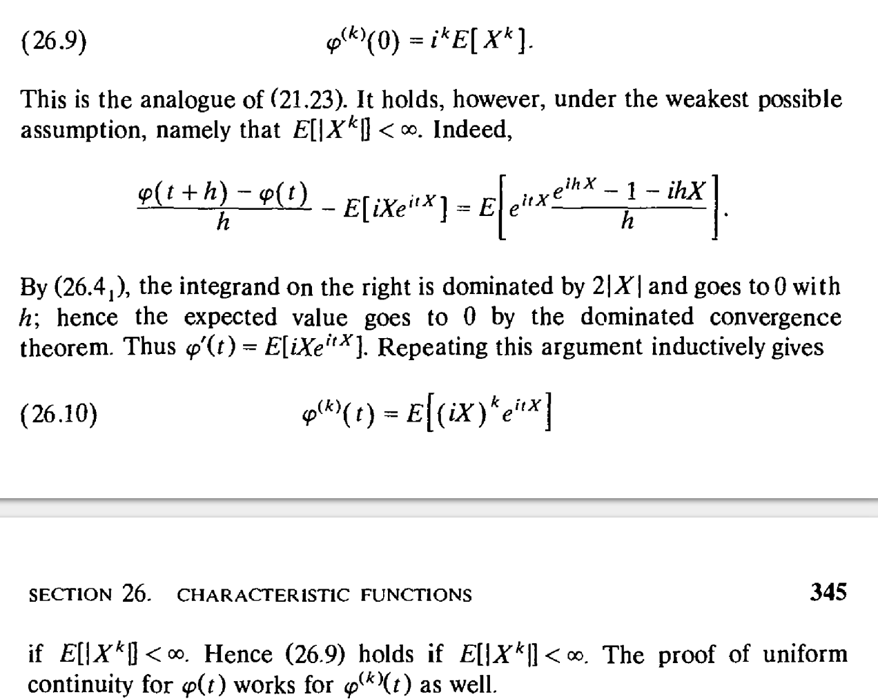
This result inspires us to compute the \(k\)-th moment \(\mathbb{E}[X^k]\) by taking \(k\)-th derivative of \(\varphi\). We have shown that \(\varphi'(t) = \mathbb{E}[iXe^{itX}]\) when \(X\) is integrable. Repeating the argument can show that \(\varphi^{(k)}(t) = \mathbb{E}[(iX)^k e^{itX}]\) if \(X^k\) is integrable[6].
Corollary. If \(|X|^k\) is integrable, then \(\varphi\) is \(k\)-th differentiable and \(\varphi^{(k)}(0) = i^k \mathbb{E}[X^k]\). Moreover, the \(k\)-th derivative is bounded, uniformly continuous, and has an explicit form \(\varphi^{(k)}(t) = \mathbb{E}[(iX)^k e^{itX}]\).
Related to Weak Convergence
Finally, c.f.s are useful in studying limiting distributions. This is due to the continuity theorem. The proof utilizes the concept of tightness of measures and thus is omitted here; see, e.g., Billingsley's book (2008, pp. 349–350) or Durrett's book (2019, pp. 114–115).
Theorem (Continuity theorem). Let \(\mu_n\) and \(\mu\) be finite measures with c.f.s \(\varphi_n\) and \(\varphi\). Then \(\mu_n \Rightarrow \mu\) if and only if \(\varphi_n(t) \to \varphi(t)\) for each \(t\).
Remark. The condition requires that the limiting function \(\lim \varphi_n(t)\) is indeed a c.f. of some finite measure \(\mu\). However, it might not be true. For example, let \(\varphi_n(t) = \exp(-nt^2/2)\) be the c.f. of the Gaussian distribution \(\mathcal{N}(0, n)\). Then \(\lim \varphi_n(t) = \mathbb{1}_{\{0\}}(t)\), which is clearly not a c.f. (as any c.f. must be uniformly continuous). Thus, \(\mu_n\) does not converge weakly.
The continuity theorem relates the pointwise convergence of c.f.s with the weak convergence of probability measures. In the following section, we will use it to study the limiting distribution of sum of i.i.d. random variables through studying the limiting c.f., as it is much easier to work with product of c.f.s than the convolution of distributions.
Central Limit Theorem and Gaussian Distribution
With the help of c.f.s, it is not hard to find out the sum of i.i.d. random variables follows a Gaussian distribution. Let \(X_n\) be i.i.d. random variables with mean \(\mu\) and finite variance \(\sigma^2 < \infty\). Let \[ Z_n = \frac{\sum_{k=1}^n X_k - n\mu}{\sqrt{n}\sigma}. \] Now we show that the limiting distribution of \(Z_n\) is the standard Gaussian distribution \(\mathcal{N}(0, 1)\).
Let \(Y_n = (X_n - \mu) / \sigma\). Then \(Y_n\) are i.i.d. random variables with mean 0 and variance 1. Let \(\varphi_n\) be their c.f.s. Of course, as \(Y_n\) are i.i.d., their c.f. are the same \(\varphi_n \equiv \varphi\). By the continuity theorem, it is sufficient to show the c.f. of \(Z_n\) converges to \(\exp(-t^2/2)\). \[ \mathbb{E}[\exp(itZ_n)] = \mathbb{E}\biggl[ \exp\biggl( it \frac{\sum_{k=1}^n Y_k}{\sqrt{n}} \biggr) \biggr] = \prod_{k=1}^n \mathbb{E}\biggl[\exp\biggl(it \frac{Y_k}{\sqrt{n}} \biggr) \biggr] = \biggl[\varphi\biggl(\frac{t}{\sqrt{n}}\biggr)\biggr]^n. \] As \(Y_k\) has mean 0 and finite variance 1, it must be square integrable. Thus, its c.f. has Taylor expansion \[ \varphi(t) = 1 - \frac{1}{2}t^2 + o(t^2).\] Hence, we can continue to caculate the c.f. of \(Z_n\). \[ \mathbb{E}[\exp(itZ_n)] = \biggl[\varphi\biggl(\frac{t}{\sqrt{n}}\biggr)\biggr]^n = \biggl[ 1 - \frac{t^2}{2n} + o\biggl(\frac{t^2}{n}\biggr) \biggr]^n \to \exp(-t^2/2). \] The final limit exists as \((1 + c/n + o(1/n))^n \to e^c\) for all real number \(c\)[7].
Theorem. (Central limit theorem). Let \(X_1, X_2, \ldots\) be i.i.d. random variables with mean \(\mu\) and positive finite variance \(\sigma^2\). Then \[ \frac{\sum_{k=1}^nX_k - n\mu}{\sigma\sqrt{n}} \Rightarrow \mathcal{N}(0, 1). \]
Footnotes:
For any Borel set \(B\), there is (the last equality holds because of independence) \[ \mu_{X_1+X_2}(B) = \mathbb{P}(X_1 + X_2 \in B) = \mathbb{E}[\mathbb{1}(X_1 + X_2 \in B)] = \int \mathbb{1}(x_1 + x_2 \in B) \, \mu_{X_1}(dx_1) \mu_{X_2}(dx_2). \] In general, the convolution of two finite measure is defined by \[ \mu_1 \star \mu_2 (B) := \int \mathbb{1}_B(x+y) \, \mu_1(dx) \mu_2(dy). \] The convolution theorem states that the c.f. of \(\mu_1 \star \mu_2\) is exactly \(\varphi_{\mu_1}(t) \varphi_{\mu_2}(t)\). For a direct proof, see Schilling's book (2017, p. 221).
The normal density function with mean \(it\) and variance 1 indeed integrals to 1 for all real \(t\), but this conclusion requires proof. The rigorous treatment is showing the c.f. of the standard normal distribution is indeed \(e^{-t^2/2}\). As \(X\) is integrable, the c.f. is continuously differentiable and
$$ \begin{aligned} \varphi'(t) &= \mathbb{E}[iXe^{itX}] \\ &= \int ix e^{itx} \frac{1}{\sqrt{2\pi}} e^{-x^2/2} \, dx \\ &= \int -i e^{itx} \, d\frac{1}{\sqrt{2\pi}} e^{-x^2/2} \\ &= -\int t e^{itx} \frac{1}{\sqrt{2\pi}} e^{-x^2/2} \, dx \ &= -t \varphi(t). \end{aligned} $$Let \(\xi(t) = \varphi(t) \exp(t^2/2)\). Then \(\xi(0) = 1\) and \(\xi'(t) = [\varphi'(t) + t\varphi(t)]\exp(t^2/2) \equiv 0\). Hence, \(\xi(t) = \varphi(t) \exp(t^2/2) \equiv 1\).
In order to see this, we prove the following lemma first.
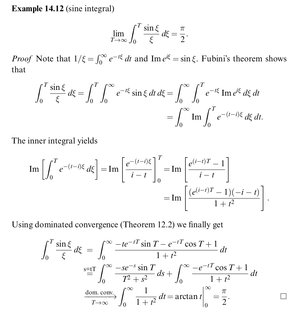
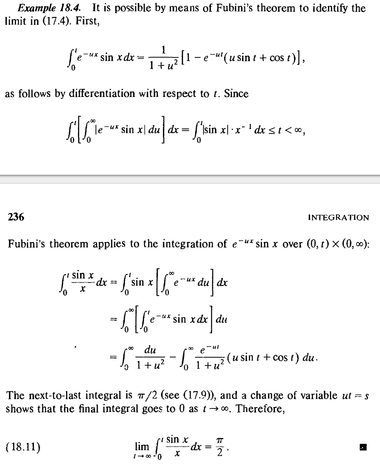
Lemma. The sinc function \(\frac{\sin x}{x}\) is not integrable but its improper Riemann integral exists \[\lim_{T\to\infty} \int_{-T}^T \frac{\sin x}{x} \, dx = \pi.\]
This sinc function is a sequence of "bumps" of decreasing size. The \(n\)-th "bump" bounds area on the order of \(1/n\), but \(\sum 1/n = \infty\). To see this,
$$ \begin{aligned} \int \biggl| \frac{\sin x}{x} \biggr| \, dx &= 2\int_0^\infty \frac{|\sin x|}{x} \, dx \\ &= 2\sum_{k=0}^\infty \int_{k\pi}^{(k+1)\pi} \frac{|\sin x|}{x} \, dx \\ &\geq 2\sum_{k=0}^\infty \int_{k\pi}^{(k+1)\pi} \frac{|\sin x|}{(k+1)\pi} \, dx \\ &= \frac{4}{\pi} \sum_{k=0}^\infty \frac{1}{k+1}. \end{aligned} $$This concludes that \(\frac{\sin x}{x}\) is not integrable. Nevertheless, the improper Riemann integral exists and equals \(\pi\); see, e.g., Schilling's book (2017, p. 145) or Billingsley's book (2008, pp. 235–236).
Let \(S(T) = \int_0^T \frac{\sin x}{x} \, dx\). Then \(S(T) \to \pi/2\). Moreover, there exists a constant \(M\) such that \(|S(T)| \leq M\). Indeed, as \(S(T) \to \pi/2\), there exists \(T_0 > 0\) such that \(|S(T)| \leq \pi\) for all \(T \geq T_0\). For \(T < T_0\), there is \(|S(T)| \leq \int_0^{T_0} |\sin x| / |x| \, dx \leq T_0\). Hence, \(|S(T)| \leq \max(T_0, \pi)\).
Now we can discuss the boundness and convergence result of \(R(x; T)\). Consider \(f(\xi, t) = e^{it\xi} \mathbb{1}(x - b \leq \xi \leq x - a)\). Clearly, \(f(\xi, t)\) is integrable on the product space \(\mathbb{R} \times [-T, T]\). Hence, we can apply Fubini's theorem to interchange the order of integrals.
$$ \begin{aligned} R(x; T) &:= \frac{1}{2\pi} \int_{-T}^T \frac{e^{it(x-a)} - e^{it(x-b)}}{it} \, dt \\ &= \frac{1}{2\pi} \int_{-T}^T dt \int d\xi \, e^{it\xi} \mathbb{1}(x - b \leq \xi \leq x - a) \\ &= \frac{1}{2\pi} \int d\xi \int_{-T}^T dt \, e^{it\xi} \mathbb{1}(x - b \leq \xi \leq x - a) \\ &= \frac{1}{\pi} \int_{x-b}^{x-a} \frac{\sin (T\xi)}{\xi} \, d\xi \\ &= \frac{1}{\pi}[\operatorname{sgn} (x-a) S(T|x-a|) - \operatorname{sgn} (x-b) S(T|x-b|)]. \end{aligned} $$Here we use the fact that for any real number \(c\), the integral \(\int_0^c \frac{\sin Tx}{x} \, dx = \operatorname{sgn}(c) S(T|c|)\). As \(|S(T)| \leq M\) for some constant \(M\), we conclude that \(|R(x; T)| \leq 2M/\pi\). Moreover, as \(T \to \infty\), \[ R(x; T) \to \begin{cases} 1, &\quad a < x < b, \\ 1/2, &\quad x = a \text{ or } x = b, \\ 0, &\quad x < a \text{ or } x > b. \end{cases} \]
In general, by integration by parts
$$ \begin{aligned} \int_0^x \frac{(x - t)^n}{n!} f^{(n+1)}(t) \, dt &= \int_0^x \frac{(x - t)^n}{n!} \, df^{(n)}(t) \\ &= -\frac{x^n}{n!}f^{(n)}(0) + \int_0^x \frac{(x-t)^{n-1}}{(n-1)!} f^{(n)}(t) \, dt \\ &= \cdots \\ &= -\frac{x^n}{n!}f^{(n)}(0) - \cdots - \frac{x^2}{2}f''(0) - xf'(0) + \int_0^x f'(t) \, dt \\ &= f(x) - f(0) - \sum_{k=1}^n \frac{f^{(k)}(0)}{k!} x^k. \end{aligned} $$Assume \(\xi < 0\). Then,
$$ \begin{aligned} \biggl| e^{i\xi} - 1 - \sum_{k=1}^n \frac{i^k}{k!} \xi^k \biggr| &= \biggl| \int_0^\xi \frac{(\xi -t)^n}{n!} i^{n+1} e^{it} \, dt \biggr| \\ &= \biggl| \int_\xi^0 \frac{(\xi -t)^n}{n!} i^{n+1} e^{it} \, dt \biggr| \\ &\leq \int_\xi^0 \frac{|\xi -t|^n}{n!} \, dt \\ &= \int_\xi^0 \frac{(t-\xi)^n}{n!} \, dt \\ &= \frac{(-\xi)^{n+1}}{(n+1)!}. \end{aligned} $$See, e.g., Billingsley's book (2008, pp. 344–345).
Taking log on the limit yields \[ \lim_{n\to\infty} \frac{\log(1 + c/n + o(1/n))}{1/n} = \lim_{n\to\infty} \frac{\log(1 + c/n + o(1/n))}{c/n + o(1/n)} \cdot \frac{c/n + o(1/n)}{1/n} = c. \]