17 Mar 2024

Strong Law of Large Numbers

We all know that probability can be interpreted as frequency, but behind it there is an important theorem in probability and statistic theory, called Strong Law of Large Numbers (SLLN). It states that the emprical mean, i.e., the mean of samples, will converge to the expectation of the distribution almost surely. Monte Carlo integration is actually a direct application of SLLN.

In this post, we first review the tossing coin example and prove this convergence in a probability manner rigorously. Then we review the SLLN theorem (i.i.d. case) and two applications, Monte Carlo integration and Bernstein's theorem. The former is an important numerical method for estimating integrals, and the latter specifies explicitly an approximating sequence to uniformly approximate any continuous function on a bounded interval with polynomials. Finally, we discuss additional theoretical results relevant to the SLLN, along with a brief outline of the proof for the SLLN theorem (i.i.d. case).

Throughout this post, for a given sequence $(a_n)$ we denote the cumulative average by $\bar{a}_n := \frac{1}{n} \sum_{k=1}^n a_k$.

Tossing a Coin: Probability as Frequency

Perhaps all of us start learning about probability by this example: if we toss a fair coin repeatly then the frequency of heads will tend to 1/2, which is the probability of a head occurring. But can we characterize this "convergence" behavior?

Let the sample space $\Omega$ be $\{0, 1\}^\mathbb{N}$, the set of infinite series with value 0 or 1. Let $X_n(\omega)$ be the $n$-th value of the series corresponding to $\omega \in \Omega$. Then clearly $X_n$ are i.i.d. r.v.s. with mean $\mathbb{E}[X_n]=1/2$. By the Strong Law of Large Numbers (SLLN), the empirical mean $\bar{X}_n = \frac{1}{n} \sum_{k=1}^n X_k$ (i.e., the frequency of heads) converges to the expectation almost surely.

For the example of tossing a coin, the conclusion can be proved easily, as the $k$-th moment always exists, $\mathbb{E}[X_n^k] = \mathbb{P}(X_n = 1) = 1/2$. To prove the almost surely convergence, we can estimate the probability of the event that the difference between the emprical mean $\bar{X}_n$ and the expectation 1/2 is larger than any positive $\epsilon$ by Markov inequality¹ \[ \mathbb{P}(|\bar{X}_n - 1/2| > \epsilon) \leq \frac{1}{\epsilon^4} \mathbb{E}[|\bar{X}_n - 1/2|^4] \leq \frac{3}{(2\epsilon)^4 n^2}. \] By Borel–Cantelli lemma, $\mathbb{P}(N_\epsilon) = 0$ for any positive $\epsilon$, where $N_\epsilon = \{|\bar{X}_n - 1/2| > \epsilon \quad \text{i.o.}\}$. Thus, for any $\omega \in N^c_\epsilon$, $|\bar{X}_n - 1/2| \leq \epsilon$ holds for all but finite many $n$'s. Taking $N = \bigcup_{\epsilon\in\mathbb{Q}_+} N_\epsilon$ concludes that $|\bar{X}_n - 1/2| \to 0$ almost surely.

Remark. The sample space $\Omega$ can be regarded as the interval $(0, 1]$ like how a real number is represented in base 2. The probability corresponds to the Lebesgue measure confined on the unit interval. In this point of view, the exception set $N$ is uncountable² but has measure 0. A number in $N^c$ is called normal number and the SLLN in this case is equivalent to $\mathbb{P}(N) = 0$, which is exactly the Borel's normal number theorem.

The essential condition in this simple proof is the finiteness of the 4-th moment. However, with advanced techniques, the existence of the expectation (possibly infinite) is enough to prove the almost surely convergence.

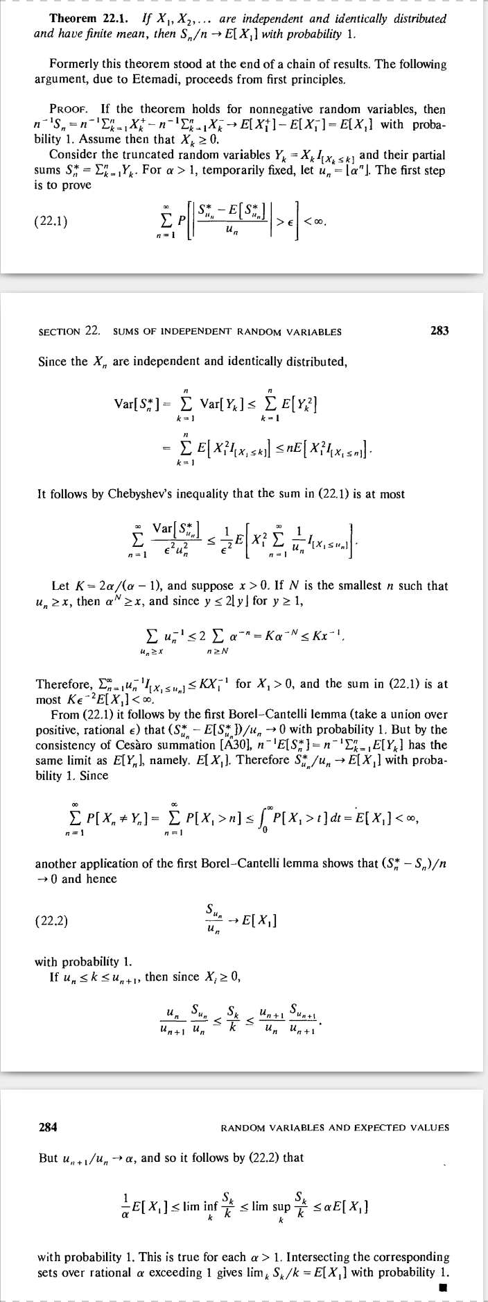
Theorem [Strong Law of Large Numbers (i.i.d. case)]. Let $(X_n)_{n=1}^\infty$ be independent and identically distributed and $\mathbb{E}[X_1]$ exists (possibly infinite), then $\bar{X}_n$ converges to $\mathbb{E}[X_1]$ almost surely.

Application: Monte Carlo Integration

Perhaps Monte Carlo Integration is one of the most promising application of SLLN. Assume we want to estimate the integral $\int_A f(x) \, dx$. Suppose we are able to sample from a reference distribution $p$ whose support $\mathcal{X} \supset A$. Hence, we can rewrite the integral as an expectation \[ \int_A f(x) \, dx = \int_\mathcal{X} f(x) \frac{\mathbb{1}_A(x)}{p(x)} \, p(x) dx = \mathbb{E}_{X \sim p}\biggl[f(X) \frac{\mathbb{1}_A(X)}{p(X)} \biggr].\] Then by sampling from $p$ to obtain a sequence of i.i.d. observations $(X_n)$, we can generate a new sequence of i.i.d. observations $(Y_n)$ where $Y_n = f(X_n) \mathbb{1}_A(X_n) / p(X_n)$. By SLLN, the empirical mean $\bar{Y}_n$ converges almost surely to its expectation, which is exactly the integral $\int_A f(x) \, dx$.

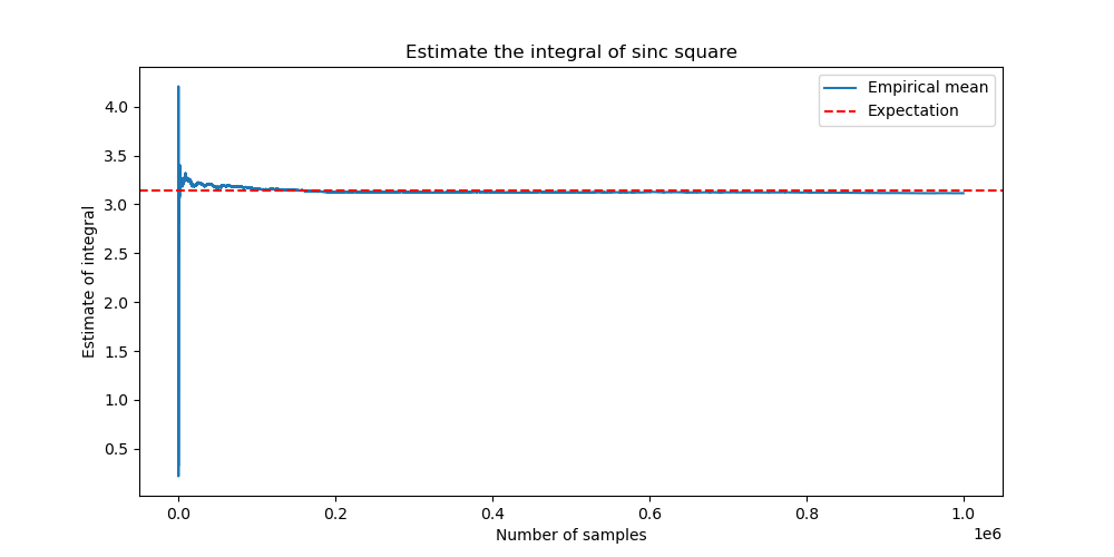
Example. Compute the integral $\int_{-\infty}^\infty \frac{\sin^2 x}{x^2} \, dx$.

Let the reference distribution $p$ be a normal distribution. Generate a sequence of Gaussian noise $(x_n)$. Compute $y_n = f(x_n) / p(x_n)$. Then the accumulative average of $(y_n)$ converges to the integral by SLLN.

A simple python code (see here) can help us visualize the above calculation. Here is the figure of the convergence of empirical mean. The horizontal line is the true value of the integral, i.e., $\pi$.

Application: Bernstein's Theorem

According to the famous Weierstrass approximation theorem, any continuous function $f$ on the compact set $[0, 1]$ can be uniformly approximated by polynomials. Interestingly, we can explicitly construct the approximating sequence with the help of SLLN.

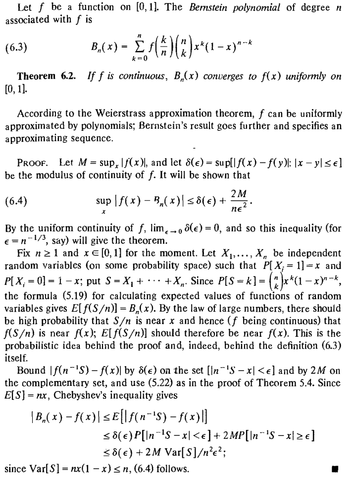
For any $x \in [0, 1]$, let $p(\cdot; x)$ be Bernoulli distribution with parameter $x$. Let $(X_n)$ be a i.i.d. sequence sampled from $p$. Then the empirical mean $\bar{X}_n$ converges to $x$ almost surely according to SLLN. By continuity, $f(\bar{X}_n) \to f(x)$ almost surely too. Noting that $f$ is bounded on $[0, 1]$, we conclude that $\mathbb{E}[f(\bar{X}_n)] \to f(x)$ by dominated convergence theorem. Surprisingly, this expectation can be expressed by a polynomial evaluated at $x$: \[ \mathbb{E}[f(\bar{X}_n)] = \sum_{k=0}^n f\biggl(\frac{k}{n}\biggr) \mathbb{P}\biggl(\sum_{i=1}^n X_i = k\biggr) = \sum_{k=0}^n f\biggl(\frac{k}{n}\biggr) {n \choose k} x^k (1-x)^{n-k} =: B_n(x; f). \] The polynomial $B_n(x; f)$ is called the Bernstein polynomial of degree $n$ associated with $f$.

Although the above argument only shows the pointwise convergence, the following Bernstein's theorem ensures that this convergence is actually uniform on $[0, 1]$³.

Theorem [Bernstein]. If $f$ is continuous, then $B_n(x; f)$ converges to $f$ uniformly on $[0, 1]$.

Proof. See here (Billingsley, 2008, p. 87).

Other Types of SLLN

SLLN states that the existence of the expectation ensures the convergence of the empirical mean. Interestingly, the converse is also true if the limit of the empirical mean is finite.

Proposition. Let $(X_n)_{n=1}^\infty$ be independent and identically distributed. If $\bar{X}_n$ converges almost surely to $\mu$, which is finite, then $\mathbb{E}[|X_1|] < \infty$ and $\mathbb{E}[X_1] = \mu$.

Proof. See Schiling's book (2017, p. 297). See also this discussion.

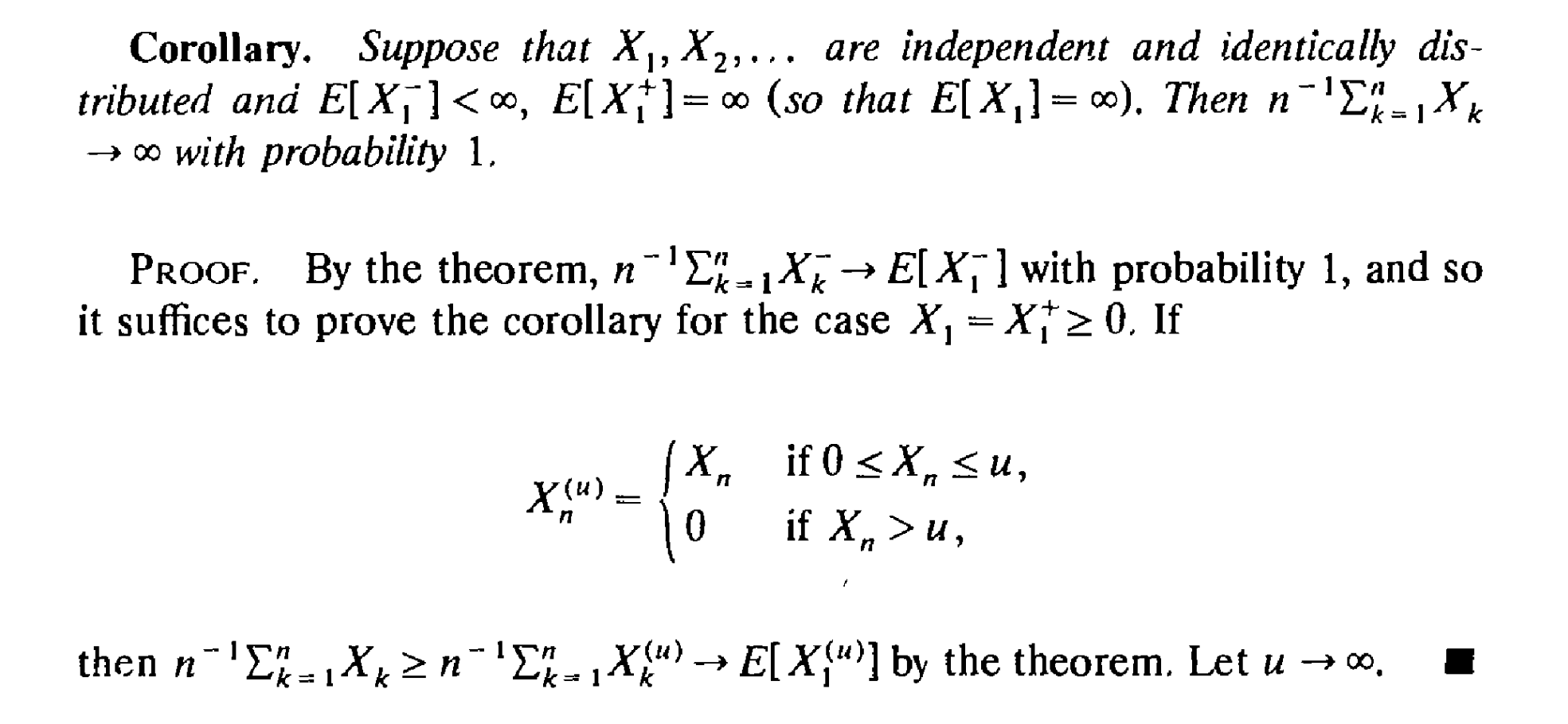
A limitation of SLLN is that it requires the existence of the expectation, which may not be guaranteed when both expectations of the positive part and the negative part are infinite. Nevertheless, it can be proved that in this case the empirical mean may diverge to infinite too.

Proposition [SLLN when mean does not exists ]. Let $(X_n)_{n=1}^\infty$ be independent and identically distributed and $\mathbb{E}[|X_1|] = \infty$, then $\limsup |\bar{X}_n| = \infty$ almost surely.

Proof. This is an exercise E4.6 Converse to SLLN in Williams's book (1991, p. 227). See also this discussion and this discussion.

Theorem [Strong Law of Large Numbers (independent case)]. Let $(X_n)_{n=1}^\infty$ be independent and $\sum \frac{\text{Var}[X_n]}{n^2} < \infty$, then $\bar{X}_n - \mathbb{E}[\bar{X}_n] \to 0$ almost surely.

Proof. See Çinlar's book (2011, p. 127). See also this lecture note.

Proof Sketch of SLLN (i.i.d. case)

The following arguments are a rephrased version from Billingsley's book (2008, pp. 282–284).

Assume $(X_n)$ are nonnegative and $\mathbb{E}[X_1] < \infty$ (later we can relax these assumptions).

Step I. Let $Y_n = X_n \mathbb{1}(X_n \leq n)$. Show it holds almost surely that \[ \bar{Y}_n - \bar{X}_n \to 0 \quad \text{and} \quad \mathbb{E}[\bar{Y}_n] - \mathbb{E}[X_1] \to 0. \]

Step II. Prove $\bar{Y}_n \to \mathbb{E}[X_1]$ almost surely. (This step is the most difficult step.)

Step III. Conclude that $\bar{X}_n \to \mathbb{E}[X_1]$ almost surely if $(X_n)$ are nonnegative and $\mathbb{E}[X_1] < \infty$.

Step IV. Prove that $\bar{X}_n \to \mathbb{E}[X_1]$ almost surely if $\mathbb{E}[X_1] < \infty$ (i.e., removing the nonnegative condition).

Step V. Prove that $\bar{X}_n \to \mathbb{E}[X_1]$ almost surely if $\mathbb{E}[X_1] = \infty$ or $\mathbb{E}[X_1] = -\infty$.

In Step II, the following technical lemma is useful: let $(a_n)$ be a positive sequence and $(\bar{a}_n)$ be its accumulative average. If a subsequence $(\bar{a}_{n_k})$ converges to $a$ and $\lim n_{k+1} / n_k = r$, then⁴ \[ \frac{1}{r}a \leq \liminf \bar{a}_n \leq \limsup \bar{a}_n \leq r a.\]

For the complete proof of Step I-IV, please see here. For the complete proof of Step V, please see here.

Footnotes:

Actually, we can show that $\mathbb{E}[|\bar{X}_n - 1/2|^4] = \frac{3}{16n^2} - \frac{1}{8n^3}$. Let $Y_n = 2X_n - 1$. Then $(Y_n)$ are i.i.d., $\mathbb{E}[Y_n^{2k+1}] = 0$ and $\mathbb{E}[Y_n^{2k}] = 1$ for all nonnegative integers $k$. Now, \[ \mathbb{E}[|\bar{X}_n - 1/2|^4] = \mathbb{E}\biggl| \frac{1}{n} \sum_{k=1}^n (X_k - 1/2) \biggr|^4 = \frac{1}{16n^4} \mathbb{E}\biggl| \sum_{k=1}^n Y_k \biggr|^4. \] In order to compute this expectation, we expand $|\sum Y_k|^4$ by multinomial theorem \[ \mathbb{E}\biggl| \sum_{k=1}^n Y_k \biggr|^4 = \sum_{|\alpha| = 4} {4 \choose \alpha} \mathbb{E}[Y^\alpha],\] where $\alpha$ is a multiindex $\alpha = (\alpha_1, \alpha_2, \ldots, \alpha_n)$ and $Y^\alpha:= \prod_{k=1}^n Y_k^{\alpha_k}$. There are five types of $\alpha$ satisfying $|\alpha|=4$, i.e., $\sum \alpha_k = 4$:

i. $\alpha$ can be sorted into $(1, 1, 1, 1, 0, \ldots, 0)$
ii. $\alpha$ can be sorted into $(2, 1, 1, 0, \ldots, 0)$
iii. $\alpha$ can be sorted into $(2, 2, 0, \ldots, 0)$
iv. $\alpha$ can be sorted into $(3, 1, 0, \ldots, 0)$
v. $\alpha$ can be sorted into $(4, 0, \ldots, 0)$

Clearly, $\mathbb{E}[Y^\alpha] \neq 0$ only for type iii and type v. In both case, $\mathbb{E}[Y^\alpha] = 1$. Type iii contains ${n \choose 2}$ indices and type v contains $n$ indices. Hence, \[ \mathbb{E}\biggl| \sum_{k=1}^n Y_k \biggr|^4 = {n \choose 2}{4 \choose {2, 2}} + n = 3n^2 - 2n. \] We can easily verify that this result is also true for $n \leq 3$.

Indeed, for any $x \in (0, 1]$, let $\omega_x = (d_1, d_2, \ldots)$ be the dyadic expansion of $x$, i.e., $x = \sum \frac{d_k}{2^k}$. Let $\omega' = (1, 1, d_1, 1, 1, d_2, \ldots)$ be defined by $\omega'_i = d_i$ if $i \mod 3 = 0$ and $\omega'_i = 1$ otherwise. Then clearly $\bar{X}_n(\omega') \geq 2/3$ for all $n$ and thus $\omega' \in N$. This shows that there is an injection map from $(0, 1]$ to $N$.

The proof is based on Chebyshev's inequality. Let $M= \sup_{x \in [0, 1]}|f(x)|$. For any $\epsilon > 0$, let $\delta(\epsilon) = \sup_{|x - y| < \epsilon, x, y \in [0, 1]} |f(x) - f(y)|$. Noting that $B_n(x; f) = \mathbb{E}[f(\bar{X}_n)]$,

$$ \begin{aligned} |B_n(x; f) - f(x) | & = |\mathbb{E}[f(\bar{X}_n)] - f(x)| \\ & \leq \mathbb{E}|f(\bar{X}_n) - f(x)| \\ & \leq \delta(\epsilon) \mathbb{P}(|\bar{X}_n - x| \leq \epsilon) + 2M \mathbb{P}(|\bar{X}_n - x| > \epsilon) \\ & \leq \delta(\epsilon) + 2M \frac{p(1-p)}{n\epsilon^2}. \end{aligned} $$

By choosing $\epsilon = (1/n)^{1/4}$, the uniform norm $\|B_n - f\|$ converges to 0 (noting that $\delta(\epsilon) \to 0$ as $f$ is uniformly continuous).

⁴

For $n_k \leq n < n_{k+1}$ (noting $a_n \geq 0$), there is \[ \frac{n_k}{n_{k+1}} \bar{a}_{n_k} \leq a_n \leq \frac{n_{k+1}}{n_{k}} \bar{a}_{n_{k+1}}. \]