Convergence in Distribution and Weak Convergence

Definition. A sequence of real-valued random variables \(\{X_n\}\) (with distribution functions \(\{F_n\}\)) is said to converge in distribution or in law to \(X\) (with distribution function \(F\)) if \(F_n(x)\) converges to \(F(x)\) at continuity points \(x\) of \(F\), i.e., \[\lim_n F_n(x) = F(x), \quad\text{for every continuity point $x$ of $F$}.\]

Remark. In this definition, it is the distribution function which matters, and there is nothing to do with the underlying probability space. So, random variables \(\{X_n\}\) may be defined on entirely different probability space.

As we all know, there is a one-to-one correspondence between distribution functions and probability measures¹. Therefore, we can define the convergence of probability measures in the same vain.

Definition. A sequence of probability measures \(\{\mu_n\}\) on the real line is said to converge weakly to a probability measure \(\mu\) if \[ \lim_n \mu_n((-\infty, x]) = \mu((-\infty, x]), \quad \text{for which $\mu(\{x\}) = 0$}.\]

Remark. Like the continuity condition in the definition of convergence in distributions, here the condition \(\mu(\{x\})=0\) is also essential. In fact, the set \((\infty, x])\) is called a \(\mu\)-continuity set if \(\mu(\{x\})=0\). If a set \(A\) is not a \(\mu\)-continuity set, then \(\lim_n\mu_n(A)\) may fail to converge to \(\mu(A)\).

Notation. We write \(X_n ⇒ X\) if \(X_n\) converge in law to \(X\). In this case, we may also write \(F_n ⇒ F\). Similarly, we write \(\mu_n ⇒ \mu\) if \(\mu_n\) converge weakly to \(\mu\).

Obviously, random variables \(X_n\) converge in law to \(X\) if and only if probability measures \(\mathbb{P}_{ X_n}\) converge weakly to \(\mathbb{P}_{X}\), i.e., \[\lim_n \mathbb{P}_{X_n}((-\infty, x]) = \mathbb{P}_{X}((-\infty, x]), \quad\text{for every $x$ such that $\mathbb{P}_X(\{x\})=0$}.\]

Example. Let \(\mu_n\) corresponds to a mass of \(1/n\) at each point \(0, \frac{1}{n}, \frac{2}{n}, \ldots, \frac{n-1}{n}\). Then it is clear that \(\mu_n\) converges weakly to \(\mu\), the Lebesgue measure confined on \([0,1]\). However, \(\mu_n(\mathbb{Q}\cap[0,1])=1\) for all \(n\) but \(\mu(\mathbb{Q}\cap[0,1])=0\).

Example. Let \(X_n\equiv a_n\) and \(X\equiv a\). Then \(F_n(x)=\mathbb{1}(x\geq a_n)\) and \(F(x)=\mathbb{1}(x\geq a)\). Clearly, \(X_n\) converges in distribution to \(X\) if and only if \(a_n\to a\). However, if \(a_n > a\) for infinite many \(n\), then \(F_n(a)\) fails to converge to \(F(a)\).

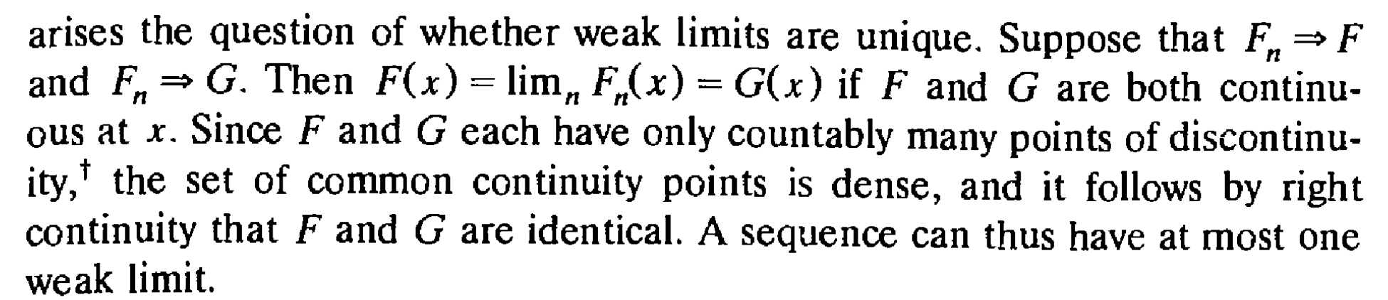
Finally, we should mention that the limit of convergence in law and weak convergence is unique. If \(F_n ⇒ F\) and \(F_n ⇒ G\), then \(F(x)=G(x)\) holds for every \(x\), including their discontinuities. Indeed, by the definition of weak convergence, \(F\) and \(G\) agree on the real line except countable points. As \(F\) and \(G\) are right continuous, they must agree on those countable points. See here for a complete proof.

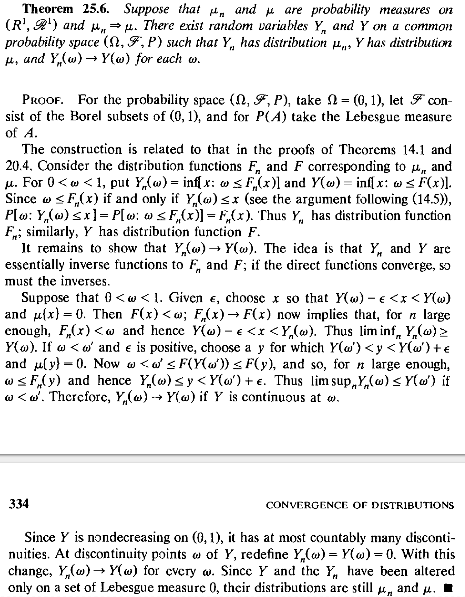
For any probability measure \(\mu_n\) on the real line, we can construct a probability space and a random variable \(Y_n\) on it such that \(Y_n\) induces \(\mu_n\). For probability measures \(\mu_n ⇒ \mu\), the following theorem states that \(Y_n\) and \(Y\) can be constructed on the same probability space, and even in such a way that \(Y_n(\omega) \to Y(\omega)\) fo every \(\omega\), which is a much stronger condition than \(Y_n ⇒ Y\).

Theorem [Skorohod]. Suppose that \(\mu_n ⇒ \mu\). Then there exists a probability space \((\Omega,\mathcal{F},\mathbb{P})\) and random variables \(Y_n\) and \(Y\) on it such that \(Y_n\) has distribution \(\mu_n\), \(Y\) has distribution \(\mu\), and \(Y_n(\omega)\to Y(\omega)\) for every \(\omega\).

Proof. The proof is constructive and based on quantile functions. See here for the complete proof. You may also want to look at this post for a brief review of quantile functions. Below is the sketch of constructing those random variables.

Let \(F_n\) and \(F\) be the distribution functions corresponding to \(\mu_n\) and \(\mu\). Let \(q_n\) and \(q\) be the corresponding quantile functions. Take the probability space on which there exists a random variable \(U\) which follows the uniform distribution on \((0,1)\). Then \(q_n(U)\) and \(q(U)\) have distribution \(\mu_n\) and \(\mu\) respectively. It can be proved that if \(F_n(x)\to F(x)\) at continuity points of \(F\) then \(q_n(u)\to q(u)\) at continuity points of \(q\). Let \(N\subset(0,1)\) be the set of discontinuity points of \(q\). Define

$$ Y_n(\omega) = \begin{cases} q_n(U(\omega)),&\quad \omega\not\in N,\\ 0,&\quad\omega\in N, \end{cases} \quad Y(\omega) = \begin{cases} q(U(\omega)),&\quad \omega\not\in N,\\ 0,&\quad\omega\in N. \end{cases} $$

Then \(Y_n\) and \(Y\) satisfy the desired properties.

Q.E.D.

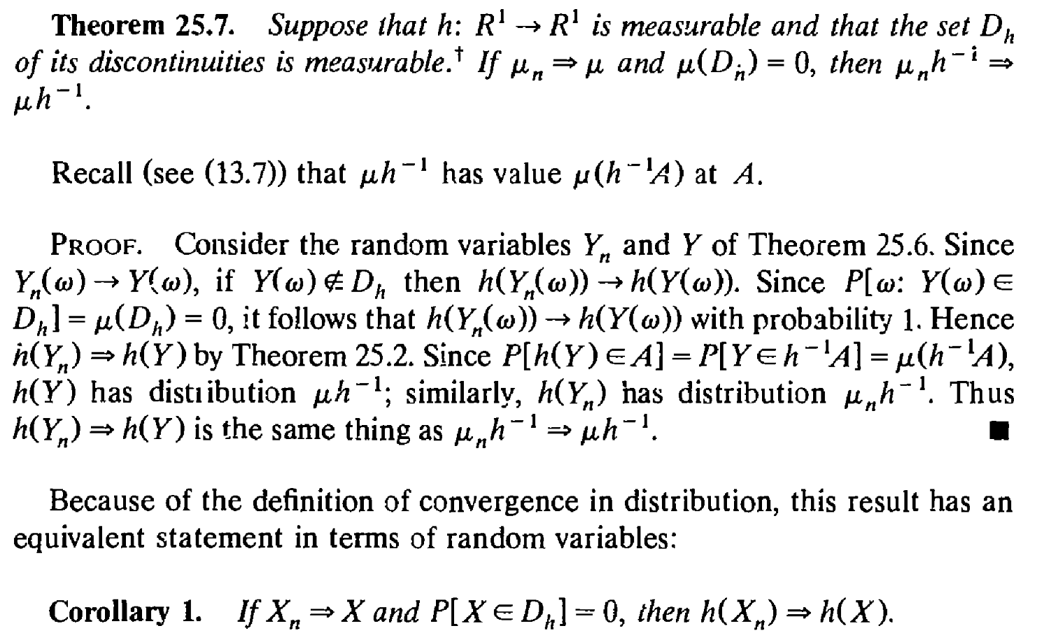
Corollary 1. If \(X_n ⇒ X\) and \(\mathbb{P}(X \in D_h)=0\), then \(h(X_n) ⇒ h(X)\). Here, \(D_h\) is the set of discontinuity points of the measurable function \(h\).

Proof. See here.

Corollary 2. If \(X_n ⇒ a\) and \(h\) is continuous at \(a\), then \(h(X_n) ⇒ h(a)\).

Definition. A set \(A\) is a \(\mu\)-continuity set if it is a Borel set and \(\mu(\partial A)=0\). Here, the boundary \(\partial A\) is the closure of \(A\) minus its interior.

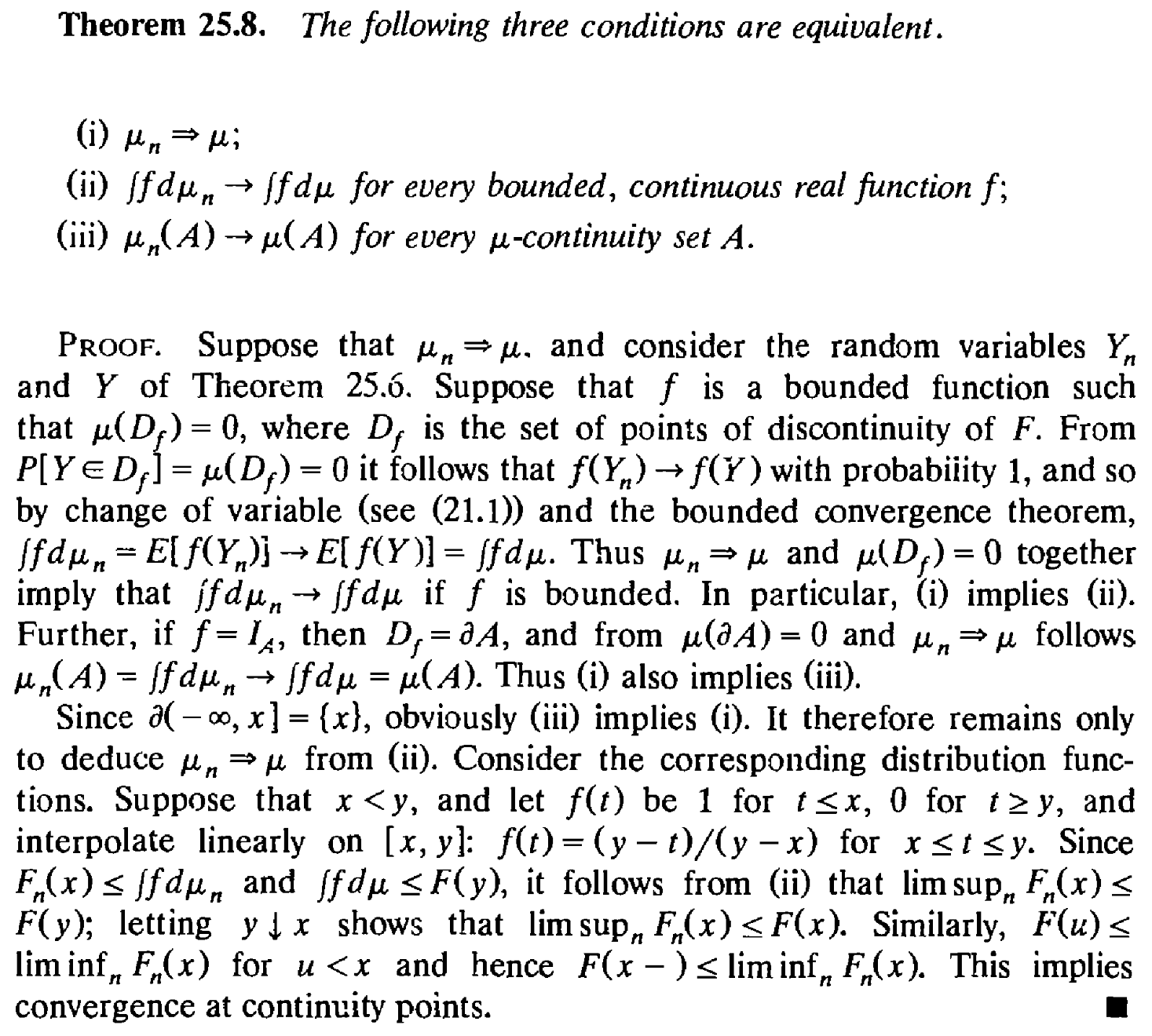
Theorem. The following conditions are equivalent.

1. \(\mu_n ⇒\mu\);
2. \(\int f\,d\mu_n \to \int f\,d\mu\) for every bounded and continuous real function \(f\);
3. \(\int f\,d\mu_n \to \int f\,d\mu\) for every bounded and uniformly continuous real function \(f\);
4. \(\mu_n(A)\to \mu(A)\) for every \(\mu\)-continuity set \(A\).

Those equivalent statements can be used to define the weak convergence of probability measures on general Polish spaces, not limited to the real line. See Parthasarathy's book Probability Measures on Metric Spaces for a complete discussion

Proof. See here. The basic ideas in the proof are listed below.

1. Clearly 4) ⇒ 1) and 2) ⇒ 3).
2. If 1) holds, then we can prove for any bounded real function on \(\mathbb{R}\) such that the discontinuity points of \(f\) is a \(\mu\)-null set there is \(\int f\,d\mu_n\to\int f\,d\mu\). Hence, 1) ⇒ 2), 1) ⇒ 3), 1) ⇒ 4).
3. Then it remains to show 3) ⇒ 1). For any \(x\in\mathbb{R}\) and \(ϵ > 0\), pick a bounded and uniformly continuous function \(f_ϵ\) such that \(\mathbb{1}_{(-\infty, x]} \leq f_ϵ \leq \mathbb{1}_{(-\infty, x+\epsilon]}\) on the real line (e.g., the function \(f_ϵ\) can be constructed by piecewise linear function). Then \(\int f_ϵ\,d\mu_n\to\int f_ϵ\,d\mu\) implies \(\limsup \mu_n((-\infty,x]) \leq \mu((-\infty,x+ϵ])\). Similarly, there is \(\mu((-\infty, x-ϵ]) \leq \liminf \mu_n((-\infty,x])\). Then \(\mu_nu((-\infty,x])\to\mu((-\infty,x])\) when \(\mu(\{x\})=0\).

Q.E.D.